Read the manual below or download the PDF.
If you are looking for the SHARC 3.0 manual, download the PDF here instead.
SHARC: Surface Hopping in the Adiabatic Representation Including Arbitrary Couplings-Manual
Contents
1 Introduction
1.1 Capabilities
1.1.1 New features in SHARC Version 4.0
1.1.2 New features in SHARC Version 4.1
1.2 References
1.3 Authors
1.3.1 Eternal list of contributors
1.3.2 List of contributors to SHARC 4
1.4 Suggestions and Bug Reports
1.5 Notation in this Manual
1.6 Terms of Use
2 Installation
2.1 How To Obtain
2.2 Installation
2.2.1 Libraries
2.2.2 Compilation of SHARC’s binaries
2.2.3 WFOVERLAP Program
2.2.4 Test Suite
2.2.5 Additional Programs
2.2.6 Quantum Chemistry Programs
3 Execution
3.1 Running a single trajectory
3.1.1 Input files
3.1.2 Running the dynamics code
3.1.3 Output files
3.2 Typical workflow for an ensemble of trajectories
3.2.1 Initial condition generation
3.2.2 Setting up the dynamics simulations
3.2.3 Running the dynamics simulations
3.2.4 Analysis of the dynamics results
3.3 Programs and Scripts of the SHARC Suite
3.3.1 Setup and Preparation
3.3.2 Trajectory Running and Management
3.3.3 Analysis
3.3.4 Others
3.3.5 Interfaces
3.4 The SHARC dynamics drivers
3.4.1 Original driver: sharc.x
3.4.2 PySHARC driver: driver.py
4 Input files
4.1 Main input file
4.1.1 General remarks
4.1.2 Input keywords
4.1.3 Detailed Description of the Keywords
4.1.4 Example
4.2 Geometry file
4.3 Velocity file
4.4 Coefficient file
4.5 Laser file
4.6 Atom mask file
4.7 RATTLE file
4.8 Frozen atoms file
4.9 Thermostat settings file
5 Output files
5.1 Log file: output.log
5.2 Listing file: output.lis
5.3 Data file: output.dat
5.3.1 Specification of the data file
5.4 Data file in NetCDF format: : output.dat.nc
5.5 Separate nuclear data file in NetCDF format: output_NUC.dat.nc
5.6 XYZ file: output.xyz
6 Interfaces
6.0.1 Overview over Interfaces
6.0.2 Associated File Names and Example Directory
6.0.3 Generic keywords in resource files of many interfaces
6.0.4 Interface development guide
6.1 Do-Nothing Interface
6.2 QMout Interface
6.3 Analytical PESs Interface
6.3.1 Parametrization
6.3.2 Template file: ANALYTICAL.template
6.3.3 Template file: ANALYTICAL.resources
6.3.4 During setup
6.4 LVC Interface
6.4.1 Input files
6.4.2 Resource file
6.4.3 During setup
6.4.4 Template File Setup: setup_LVCparam.py, create_LVCparam.py, modify_LVC_template.py
6.4.5 Vibronic spectra from VC models: FCClasses_from_LVC.py
6.5 SPaiNN Interface
6.5.1 Template file: SPAINN.template
6.5.2 Resource file: SPAINN.resources
6.5.3 During setup
6.6 SCHNARC Interface
6.6.1 Template file: SCHNARC.template
6.6.2 Template file: SCHNARC.template
6.6.3 During setup
6.7 OpenMM Interface
6.7.1 Template file
6.7.2 Resource file
6.7.3 During setup
6.8 NaI Interface
6.8.1 Template file
6.8.2 Resource file
6.8.3 During setup
6.8.4 Analytical model
6.9 GAUSSIAN Interface
6.9.1 Template file: GAUSSIAN.template
6.9.2 Resource file: GAUSSIAN.resources
6.9.3 During setup
6.9.4 Extracting normal modes: GAUSSIAN_freq.py
6.10 ORCA Interface
6.10.1 Template file: ORCA.template
6.10.2 Resource file: ORCA.resources
6.10.3 During setup
6.10.4 Extracting normal modes: ORCA_hess_freq.py
6.11 BASIC ORCA Interface
6.11.1 Template file: BASICORCA.template
6.11.2 Resource file: BASICORCA.resources
6.11.3 During setup
6.12 NWCHEM Interface
6.12.1 Template file: NWCHEM.template
6.12.2 Resource file: NWCHEM.resources
6.12.3 During setup
6.13 VASP Interface
6.13.1 Template file: VASP.template
6.13.2 Resource file: VASP.resources
6.13.3 During setup
6.13.4 Extracting normal modes: vasp_to_molden.py
6.13.5 Further comments:
6.14 Turbomole Interface
6.14.1 Template file: TURBOMOLE.template
6.14.2 Resource file: TURBOMOLE.resources
6.14.3 During setup
6.15 OPENMOLCAS Interface
6.15.1 Template file: MOLCAS.template
6.15.2 Resource file: MOLCAS.resources
6.15.3 During setup
6.15.4 Template file generator: molcas_input.py
6.16 MNDO Interface
6.16.1 Template file: MNDO.template
6.16.2 Resource file: MNDO.resources
6.16.3 During setup
6.17 MOPAC-PI Interface
6.17.1 Template file: MOPACPI.template
6.17.2 Resource file: MOPACPI.resources
6.17.3 Reparametrized Hamiltonians, definition of microstates and additional potentials: ext_param
6.17.4 QM/MM force field files
6.17.5 QM/MM connection table file: MOPACPI_tnk.xyz
6.17.6 QM/MM force field file: e.g. oplsaa.prm
6.17.7 QM/MM additional force field definition file: MOPACPI_tnk.key
6.17.8 During setup
6.18 TEQUILA Interface
6.18.1 Template file: TEQUILA.template
6.18.2 Resource file: TEQUILA.resources
6.18.3 During setup
6.19 LEGACY Interface
6.19.1 Template file: LEGACY.template
6.19.2 Resource file: LEGACY.resources
6.19.3 During setup
6.20 AMS-ADF Interface
6.20.1 Template file: AMS_ADF.template
6.20.2 Resource file: AMS_ADF.resources
6.20.3 During setup
6.20.4 Frequencies converter: AMS_ADF_freq.py
6.21 COLUMBUS Interface
6.21.1 Template input
6.21.2 Resource file: COLUMBUS.resources
6.21.3 Template setup
6.21.4 During setup
6.22 BAGEL Interface
6.22.1 Template file: BAGEL.template
6.22.2 Resource file: BAGEL.resources
6.22.3 During setup
6.23 MOLPRO Interface
6.23.1 Template file: MOLPRO.template
6.23.2 Resource file: MOLPRO.resources
6.23.3 Error checking
6.23.4 Things to keep in mind
6.23.5 During setup
6.23.6 Molpro input generator: molpro_input.py
6.24 PySCF Interface
6.24.1 Template file: PYSCF.template
6.24.2 Resource file: PYSCF.resources
6.24.3 During setup
6.25 ASE Database Interface
6.25.1 Template file: ASE_DB.template
6.25.2 During setup
6.26 Umbrella Sampling Interface
6.26.1 Template file: UMBRELLA.template
6.26.2 Restraints file
6.26.3 Resource file: UMBRELLA.resources
6.26.4 During setup
6.27 Droplet Potential Interface
6.27.1 Template file: DROPLET.template
6.27.2 Resource file: DROPLET.resources
6.27.3 During setup
6.28 Classical Path Approximation (CPA) Interface
6.28.1 Template file: CPA.template
6.28.2 Resource file: CPA.resources
6.28.3 During setup
6.29 Numerical Differentiation Interface
6.29.1 Template file: NUMDIFF.template
6.29.2 Resource file: NUMDIFF.resources
6.29.3 During setup
6.30 QM/MM Interface
6.30.1 Template file: QMMM.template
6.30.2 Resource file: QMMM.resources
6.30.3 Connectivity and QM/MM type file: QMMM.table
6.30.4 During setup
6.31 ECI Interface
6.31.1 Theory and implementation
6.31.2 QM directory of ECI interface
6.31.3 Template file: ECI.template
6.31.4 Resources file: ECI.resources
6.31.5 Standard output of SHARC_ECI.py
6.31.6 During setup
6.32 Adaptive Sampling Interface
6.32.1 Template file: ADAPTIVE.template
6.32.2 Resources file: ADAPTIVE.resources
6.32.3 During setup
6.33 Fallback Interface
6.33.1 Template file: FALLBACK.template
6.33.2 During setup
6.34 File-based Interface Specifications
6.34.1 QM.in Specification
6.34.2 QM.out Specification
6.34.3 Further Specifications
6.34.4 Save Directory Specification
6.35 The WFOVERLAP Program
6.35.1 Installation
6.35.2 Workflow
6.35.3 Calling the program
6.35.4 Input data
6.35.5 Output
7 Auxilliary Scripts
7.1 Wigner Distribution Sampling: wigner.py
7.1.1 Usage
7.1.2 Normal mode types
7.1.3 Non-default masses
7.1.4 Sampling at finite temperatures
7.1.5 Output
7.2 Vibrational State Selected Sampling: wigner_state_selected.py
7.2.1 Usage
7.2.2 Major options
7.2.3 Template
7.2.4 Normal mode types
7.2.5 Non-default masses
7.2.6 Output
7.3 Initial condition for collision dynamics: bimolecular_collision.py
7.3.1 Usage
7.3.2 Usage
7.4 AMBER Trajectory Sampling: amber_to_initconds.py
7.4.1 Usage
7.4.2 Time Step
7.4.3 Atom Types and Masses
7.4.4 Output
7.5 VASP Trajectory Sampling: vasp_to_initconds.py
7.5.1 Usage
7.5.2 Output
7.6 SHARC Trajectory Sampling: sharctraj_to_initconds.py
7.6.1 Usage
7.6.2 Random Picking of Time Step
7.6.3 Output
7.7 Creating an XYZ file from an Amber restart file: restartnc_to_xyz.py
7.7.1 Usage
7.7.2 Input
7.7.3 Output
7.8 Creating an XYZ file from a SHARC trajectory: sharctraj_to_xyz.py
7.8.1 Usage
7.8.2 Input
7.8.3 Output
7.9 Setup of Initial Calculations: setup_init.py
7.9.1 Usage
7.9.2 Input
7.9.3 Interface-specific input
7.9.4 Input for Run Scripts
7.9.5 Output
7.10 Excitation Selection: excite.py
7.10.1 Usage
7.10.2 Input
7.10.3 Output
7.10.4 Specification of the initconds.excited file format
7.11 Calculation of Absorption Spectra: spectrum.py
7.11.1 Input
7.11.2 Output
7.11.3 Error Analysis
7.12 Laser field generation: laser.x
7.12.1 Usage
7.12.2 Input
7.13 Prepare electron-only dynamics simulations: setup_laser_excitation.py
7.13.1 Usage
7.13.2 Input
7.13.3 Output
7.14 Exciting with electron-only dynamics simulations: excite_laser_excitation.py
7.14.1 Usage
7.14.2 Input
7.14.3 Output
7.15 Select initial states with the promoted density approach: excite_with_promdens.py
7.15.1 Usage
7.15.2 Input
7.15.3 Output
7.16 Preparing QM/MM calculations: setup_from_prmtop.py
7.16.1 Usage
7.16.2 Input
7.16.3 Output
7.17 Preparing RESP fits: resp_memory_estimator.py
7.17.1 Usage
7.17.2 Input
7.17.3 Output
7.18 Setup of Trajectories: setup_traj.py
7.18.1 Input
7.18.2 Interface-specific input
7.18.3 Running and output control
7.18.4 Run script setup
7.18.5 Output
7.19 File transfer: retrieve.sh
7.20 Resetting trajectories: clean_traj.sh
7.20.1 Usage
7.21 Ensemble Diagnostics Tool: diagnostics.py
7.21.1 Usage
7.21.2 Input
7.22 Data Extractor: data_extractor.x
7.22.1 Usage
7.22.2 Output
7.23 Data Extractor for NetCDF: data_extractor_NetCDF.x
7.23.1 Usage
7.23.2 Output
7.24 Data Converter for NetCDF: data_converter.x
7.24.1 Usage
7.24.2 Output
7.25 Data Converter from NetCDF to ASCII: data_converter_to_ASCII.x
7.25.1 Usage
7.25.2 Output
7.26 Data Converter from NetCDF nuclear files to XYZ: data_extractor_NUC_xyz.py
7.26.1 Usage
7.26.2 Options
7.26.3 Output
7.27 Plotting the Extracted Data: make_gnuscript.py
7.28 Internal Coordinates Analysis: geo.py
7.28.1 Input
7.28.2 Options
7.29 Normal Mode Analysis: geo_NM.py
7.29.1 Input
7.29.2 Output Format
7.30 Apply the time shift to the listing file: shift_output_lis.py
7.30.1 Usage
7.31 Calculation of Ensemble Populations: populations.py
7.31.1 Usage
7.31.2 Output
7.32 Calculation of Numbers of Hops: transition.py
7.32.1 Usage
7.33 Fitting population data to kinetic models: make_fit.py
7.33.1 Usage
7.33.2 Input
7.33.3 Output
7.34 Obtaining Special Geometries: crossing.py
7.34.1 Usage
7.34.2 Output
7.35 Essential Dynamics Analysis: trajana_essdyn.py
7.35.1 Usage
7.35.2 Input
7.35.3 Output
7.36 General Data Analysis: data_collector.py
7.36.1 Usage
7.36.2 Input
7.36.3 Output
7.37 Delay time distributions: delay_time.py
7.37.1 Usage
7.37.2 Input
7.37.3 Output
7.38 Handling large sets of coordinate data: align_and_reorder_traj.py
7.38.1 Usage
7.38.2 Input
7.38.3 Output
7.39 Producing radial distribution functions: frames_to_RDF.py
7.39.1 Usage
7.39.2 Input
7.39.3 Options
7.39.4 Output
7.39.5 Obtaining mask files
7.40 Producing 3D distributions: frames_to_dx.py
7.40.1 Usage
7.40.2 Input
7.40.3 Options
7.40.4 Output
7.41 Computing X-ray scattering: RDF_to_scattering.py
7.41.1 Usage
7.41.2 Input
7.41.3 Options
7.41.4 Output
7.42 Merging per-time-step-data: data_merger.py
7.42.1 Usage
7.42.2 Input
7.42.3 Options
7.42.4 Output
7.43 Optimizations: otool_external and setup_orca_opt.py
7.43.1 Usage
7.43.2 Input
7.43.3 Output
7.43.4 Description of orca_External and otool_external
7.44 Single Point Calculations: setup_single_point.py
7.44.1 Usage
7.44.2 Input
7.44.3 Output
7.45 Format Data from QM.out Files: QMout_print.py
7.45.1 Usage
7.45.2 Output
8 Methods and Algorithms
8.1 Absorption Spectrum
8.2 Active and inactive states
8.3 Amdahl’s Law
8.4 Bootstrapping for Population Fits
8.5 Computing electronic populations
8.6 Damping
8.7 Decoherence
8.7.1 Energy-based decoherence
8.7.2 Augmented FSSH decoherence
8.8 Essential Dynamics Analysis
8.9 Excitation Selection
8.9.1 Excitation Selection with Diabatization
8.10 Global fits and kinetic models
8.10.1 Reaction networks
8.10.2 Kinetic models
8.10.3 Global fit
8.11 Gradient transformation
8.11.1 Nuclear gradient tensor transformation scheme
8.11.2 Time derivative matrix transformation scheme
8.11.3 Dipole moment derivatives
8.12 Internal coordinates definitions
8.13 Kinetic energy adjustments
8.13.1 Reflection for frustrated hops
8.13.2 Choices of momentum adjustment direction
8.14 Projection operator
8.15 Fewest switches with time uncertainty
8.16 Laser fields
8.16.1 Form of the laser field
8.16.2 Envelope functions
8.16.3 Field functions
8.16.4 Chirped pulses
8.16.5 Linear chirp without Fourier transform
8.17 Laser interactions
8.17.1 Surface Hopping with laser fields
8.18 Linear/Quadratic Vibronic Coupling Models
8.18.1 Obtaining LVC parameters from ab initio data
8.19 Normal Mode Analysis
8.20 Optimization of Crossing Points
8.21 Phase tracking
8.21.1 Phase tracking of the transformation matrix
8.21.2 Tracking of the phase of the MCH wave functions
8.22 Random initial velocities
8.23 Representations
8.23.1 Current state in MCH representation
8.24 Sampling from Wigner Distribution
8.24.1 Sampling at Non-zero Temperature
8.25 Scaling
8.26 Seeding of the RNG
8.27 Selection of gradients and nonadiabatic couplings
8.28 State ordering
8.29 Surface Hopping
8.30 Self-Consistent Potential Methods
8.30.1 Decoherence in SCP methods
8.31 Effective Nonadiabatic Coupling Vector
8.32 Velocity Verlet
8.33 Wavefunction propagation
8.33.1 Propagation using nonadiabatic couplings
8.33.2 Propagation using overlap matrices – Local diabatization
8.33.3 Propagation using overlap matrices – Norm-preserving interpolation
8.34 Time Derivative Couplings and Curvature Approximation
Chapter 1 Introduction
When a molecule is irradiated by light, a number of dynamical processes can take place, in which the molecule redistributes the energy among different electronic and vibrational degrees of freedom.
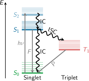
Kasha’s rule [1 ] states that radiationless transfer from higher excited singlet states to the lowest-lying excited singlet state (S1) is faster than fluorescence (F).
This radiationless transfer is called internal conversion (IC) and involves a changes between electronic states of the same multiplicity.
If a transition occurs between electronic states of different spin, the process is called intersystem crossing (ISC).
A typical ISC process is from a singlet to a triplet state, and once the lowest triplet is populated, phosphorescence (P) can take place.
In Figure 1.1 , radiative (F and P) and radiationless (IC and ISC) processes are summarized in a so-called Jablonski diagram.
The non-radiative IC and ISC processes are fundamental concepts which play a decisive role in photophysics, photochemistry, and photobiology.
IC processes are present in the excited-state dynamics of many organic and inorganic molecules, whose applications range from solar energy conversion to drug therapy.
Even many, very small molecules, for example O2 and O3, SO2, NO2 and other nitrous oxides, show efficient IC, which has important consequences in atmospheric chemistry and the study of the environment and pollution.
IC is also the first step of the biological process of visual perception, where the retinal moiety of rhodopsin absorbs a photon and non-radiatively performs a torsion around one of the double bonds, changing the conformation of the protein and inducing a neural signal.
Similarly, protection of the human body from the influence of UV light is achieved through very efficient IC in DNA, proteins and melanins.
Ultrafast IC to the electronic ground state allows quickly converting the excitation energy of the UV photons into nuclear kinetic energy, which is spread harmlessly as heat to the environment.
ISC processes are completely forbidden in the frame of the non-relativistic Schrödinger equation, but they become allowed when including spin-orbit couplings, a relativistic effect [2].
Spin-orbit coupling depends on the nuclear charge and becomes stronger for heavy atoms, therefore it is typically known as a “heavy atom” effect.
However, it has been recently recognized that even for molecules with only first- and second-row atoms, ISC might be relevant and can be competitive in time scales with IC.
A small selection of the growing number of molecules where efficient ISC in a sub-ps time scale has been predicted are SO2 [3,[4,[5], benzene [6], aromatic nitrocompounds [7] or DNA nucleobases and derivatives [8,[9,[10,[11,[12].
However, IC and ISC are also of fundamental importance in transition metal complexes, which are often used as photosensitizers or photocatalysts in various technological applications.
Overall, it can be said that the possible applications of photoinduced ultrafast dynamics are legion, and its understanding is of critical importance for many scientific investigations.
Theoretical simulations can greatly contribute to understand non-radiative processes by following the nuclear motion on the excited-state potential energy surfaces (PES) in real time.
These simulations are called excited-state dynamics simulations.
Since the Born-Oppenheimer approximation is not applicable for this kind of dynamics, nonadiabatic effects need to be incorporated into the simulations.
The principal methodology to tackle excited-state dynamics simulations is to numerically integrate the time-dependent Schrödinger equation, which is usually called full quantum dynamics simulations (QD).
Given accurate PESs, QD is able to match experimental accuracy.
However, the need for the “a priori” knowledge of the full multi-dimensional PES renders this type of simulations quickly unfeasible for more than few degrees of freedom.
Several alternative methodologies are possible to alleviate this problem.
One of the most popular ones is to use surface hopping nonadiabatic dynamics.
Surface hopping was originally devised by Tully [13] and greatly improved later by the “fewest-switches criterion”[14] and it has been reviewed extensively since then, see e.g. [15,[16,[17,[18,[19].
In surface hopping, the motion of the excited-state wave packet is approximated by the motion of an ensemble of many independent, classical trajectories. Each trajectory is at every instant of time tied to one particular PES, and the nuclear motion is integrated using the gradient of this PES. However, nonadiabatic population transfer can lead to the switching of a trajectory from one PES to another PES. This switching (also called “hopping”, which is the origin of the name “surface hopping”) is based on a stochastic algorithm, taking into account the change of the electronic population from one time step to the next one.
The advantages of the surface hopping methodology and thus its popularity are well summarized in Ref. [15]:
- The method is conceptually simple, since it is based on classical mechanics. The nuclear propagation is based on Newton’s equations and can be performed in Cartesian coordinates, avoiding any problems with curved coordinate systems as in QD.
- For the propagation of the trajectories only local information of the PESs is needed. This avoids the calculation of the full, multi-dimensional PES in advance, which is the main bottleneck of QD methods. In surface hopping dynamics, all degrees of freedom can be included in the simulation. Additionally, all necessary quantities can be calculated on-demand, usually called “on-the-fly” in this context.
- The independent trajectories can be trivially parallelized.
The strongest of these points of course is the fact that all degrees of freedom can be included easily in the calculations, allowing to describe large systems.
One should note, however, that surface hopping methods in the standard formulation [13,[14]-due to the classical nature of the trajectories-do not allow to treat some purely quantum-mechanical effects like tunneling, (tunneling for selected degrees of freedom is possible [20]). Additionally, quantum coherence between the electronic states is usually described poorly, because of the independent-trajectory ansatz. This can be treated with some ad-hoc corrections, e.g., in [21].
In the original surface hopping method, only nonadiabatic couplings are considered, only allowing for population transfer between electronic states of the same multiplicity (IC).
The SHARC methodology is a generalization of standard surface hopping since it allows to include any type of coupling. Beyond nonadiabatic couplings (for IC), spin-orbit couplings (for ISC) or interactions of dipole moments with electric fields (to explicitly describe laser-induced processes) can be included.
A number of methodologies for surface hopping including one or the other type of potential couplings have been proposed in references [22,[23,[24,[25,[26,[27,[28], but SHARC can include all types of potential couplings on the same footing.
The SHARC methodology is an extension to standard surface hopping which allows to include these kinds of couplings. The central idea of SHARC is to obtain a fully diagonal Hamiltonian, which is adiabatic with respect to all couplings. The diagonal Hamiltonian is obtained by unitary transformation of the Hamiltonian including all couplings. Surface hopping is conducted on the transformed electronic states.
This has a number of advantages over the standard surface hopping methodology, where no diagonalization is performed:
- Potential couplings (like spin-orbit couplings and laser-dipole couplings) are usually delocalized. Surface hopping, however, rests on the assumption that the couplings are localized and hence surface hops only occur in the small region where the couplings are large. Within SHARC, by transforming away the potential couplings, additional terms of nonadiabatic (kinetic) couplings arise, which are localized.
- The potential couplings have an influence on the gradients acting on the nuclei. To a good approximation, within SHARC it is possible to include this influence in the dynamics.
- When including spin-orbit couplings for states of higher multiplicity, diagonalization solves the problem of rotational invariance of the multiplet components (see [26]).
The SHARC suite of programs is an implementation of the SHARC method.
Besides the core dynamics code, it comes with a number of tools aiding in the setup, maintenance, and analysis of the trajectories.
It also provides a large suite of interfaces to many different electronic structure methods and models for excited-state potential energy surfaces.
1.1 Capabilities
The main features of the SHARC suite in Version 4.1 are:
- Non-adiabatic dynamics based on the surface hopping (SH) [29] and coherent switching with decay of mixing (CSDM) [30,[31] methodologies
- Ability to describe internal conversion and intersystem crossing with any number of states (singlets, doublets, triplets, or higher multiplicities).
- Inclusion of interactions with laser fields in the dipole approximation or including electric and magnetic fields as well as electric field gradients.
- Algorithms for stable wave function propagation in the presence of very small or very large couplings.
- Propagation using either nonadiabatic couplings vectors 〈α|[(∂)/(∂R)]|β〉, wave function overlaps 〈α(t0)|β(t)〉 (via the local diabatization procedure [21]), or based on the curvature of the potential energy surfaces [32,[33].
- Gradients including the effects of spin-orbit couplings (with the approximation that the diabatic spin-orbit couplings are slowly varying).
- A flexible, modular, nestable suite of interfaces to potential energy surface models, electronic structure softwares, and multiscale models [34].
The interface suite contains:- Fast, I/O-avoiding interfaces for analytical model potentials, linear/quadratic vibronic coupling models (optionally with electrostatic embedding) [35,[36,[37], molecular mechanics force fields ( OPENMM), and machine-learning potentials based on the FIELDSCHNET (with electrostatic embedding) or SPAINN packages;
- Interfaces for DFT and TD-DFT: GAUSSIAN 16, ORCA 5 and 6, NWChem 7.2, AMS ADF, and VASP;
- Interfaces for ADC(2) and CC2: Turbomole 7.8-8.0;
- Interfaces for SA-CASSCF and correlated multireference methods (various variants of CASPT2, MRCI, and PDFT): OPENMOLCAS 23-25, MOLPRO 2023, COLUMBUS, BAGEL, and PYSCF;
- Interfaces for semi-empirical excited-state methods: MNDO and MOPAC-PI;
- Interfaces for quantum-computing-based electronic structure using a variational quantum eigensolver: TEQUILA;
- Nestable “hybrid” interfaces for
quantum mechanics/molecular mechanics (QM/MM),
excitonic configuration interaction (ECI),
droplet/tether/harmonic restraint potentials,
classical path approximation,
adaptive sampling,
numerical differentiation,
umbrella sampling,
and storing electronic structure data.
- Energy-difference-based partial coupling approximation to speed up calculations [38].
- Energy-based decoherence correction [21], augmented-FSSH decoherence correction [39] and decay-of-mixing decoherence for SCP methods to perform CSDM or SCDM [30,[40].
- Calculation of Dyson norms for single-photon ionization spectra (for many interfaces) [41].
- On-the-fly wave function analysis with TheoDORE [42,[43,[44] (for several interfaces).
- Langevin thermostat and droplet restraining potentials.
- Suite of auxiliary Python scripts for all steps of the setup procedure: Phase space sampling from Wigner distributions or molecular dynamics trajectories, preparation of collision dynamics, initial single-point calculations, spectra simulation, selection of the initial electronic state via implicit vertical (delta pulse) excitation, the electron-only explicit (EOE) dynamics method, and the promoted density approach (PDA).
- Suite of auxiliary Python scripts for various analysis tasks: Electronic populations, nuclear motion, time-resolved spectra, solvent distributions, X-ray scattering, and several others.
- Methods to parametrize vibronic coupling models (and support for active learning of machine-learning models).
- Code to optimize minima and minimum-energy intersections (using the ORCA optimizer).
- Comprehensive tutorial.
1.1.1 New features in SHARC Version 4.0
The SHARC Version 4.0 constitutes a significant milestone in the development of the package.
The main goal was to redesign the complete framework of the communication between the SHARC dynamics driver and the electronic structure data providers.
To this end, a complete refactoring of the interfaces was carried out.
The new interfaces are developed in an object-oriented way, using inheritance to simplify development.
The communication protocol was generalized and made more rigorous.
For the user, the main advantages are (i) better performance for fast dynamics using model potentials, (ii) more systematic setup routines, and (iii) the possibility to combine and nest interfaces to achieve a broad variety of workflows.
These “interfaces that can call other interfaces” are called hybrid interfaces in SHARC.
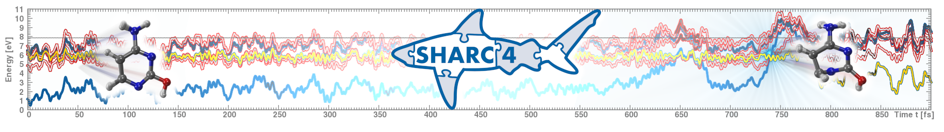
The modularity of these hybrid interfaces was the inspiration for the new SHARC logo.
The hybrid interfaces enable methods like
quantum mechanics/molecular mechanics (QM/MM) to describe solvated molecules,
excitonic configuration interaction (ECI) to describe multichromophoric systems,
adaptive sampling and automatic data storage to collect electronic structure data (for machine learning or other purposes),
automatic numerical differentiation (to get gradients, nonadiabatic couplings, or other derivatives), or
umbrella sampling for various sampling tasks.
The most important changes in SHARC 4.0 are:
- Dynamics program:
- There are now two dynamics drivers, sharc.x and driver.py.
The former driver supports all previous and new features of SHARC and uses a file-I/O-based communication with the interfaces.
The latter driver communicates with all interfaces directly in-memory, similar to the previous PySHARC modules.
Whenever we refer to PySHARC in this manual, we refer to working with driver.py. - Some features that in SHARC 3 were only available in sharc.x are now also available in driver.py (e.g., Army Ants, time uncertainty, SCP/Ehrenfest, CSDM, curvature-driven dynamics).
- Langevin thermostat and droplet restraining potential for long dynamics of liquid droplets.
- There are now two dynamics drivers, sharc.x and driver.py.
- Interfaces:
- Complete redesign, using new data classes and interface base classes, refactoring of most interfaces as given below
- New electronic structure information:
- Atom-centered multipole fit of electron densities up to quadrupole charges based on the RESP method,
- Interfaces can deliver basis set information and density matrices (handled with PySCF),
- Interfaces can receive a dedicated set of point charges to use in electrostatic embedding, and can deliver gradients and NACs on these point charges,
- Stub interfaces:
- SHARC_DO_NOTHING.py: for testing and developing
- SHARC_QMOUT.py: for frozen-nuclei trajectories
- Fast interfaces:
- SHARC_ANALYTICAL.py: for analytical PESs, redesigned around sympy,
- SHARC_LVC.py: for vibronic coupling models, redesigned and strongly improved, can do electrostatic embedding,[36,[37,[45] modify_LVC_template.py to edit LVC models,
- SHARC_SPAINN.py: new interface for machine-learning potentials based on the PaiNN architecture,
- SHARC_SCHNARC.py: new interface for machine-learning potentials based on the FieldSchnet architecture, which can do ML/MM simulations,
- SHARC_OPENMM.py: new interface for MM dynamics using AMBER prmtop files,
- Ab initio interfaces with new, SHARC4-compatible implementations:
- SHARC_GAUSSIAN.py: redesigned, can do electrostatic embedding, RESP fits, provides density matrices, GAUSSIAN_freq.py to extract frequency Molden files,
- SHARC_ORCA.py: redesigned, ORCA_hess_freq.py to extract frequency Molden files,
- SHARC_NWCHEM.py: new interface for TD-DFT in NWCHEM,
- SHARC_TURBOMOLE.py: redesigned (used to be called SHARC_RICC2.py), can do electrostatic embedding, removed dependency with ORCA for spin-orbit couplings,
- SHARC_MOLCAS.py: redesigned, can do electrostatic embedding, RESP fits, provides density matrices,
- SHARC_MNDO.py: new interface for semi-empirical MRCI based on OM2 using the MNDO code,
- SHARC_MOPACPI.py: new interface for semi-empirical MRCI using the MOPAC-PI code, which can do QM/MM with Tinker,
- SHARC_LEGACY.py: new interface that serves as a SHARC4-compatible frontend to SHARC3-style legacy interfaces,
- Legacy ab initio interfaces:
- SHARC_COLUMBUS.py, SHARC_BAGEL.py, SHARC_AMS_ADF.py: minor changes to make them compatible to SHARC_LEGACY.py,
- SHARC_MOLPRO.py: updated to work with MOLPRO 2023, minor changes to make it compatible to SHARC_LEGACY.py,
- SHARC_PYSCF.py: new SHARC3-style legacy interface for PySCF (CASSCF, MC-PDFT),
- Single-child hybrid interfaces:
- SHARC_ASE_DB.py: new single-child hybrid interface to store geometries and electronic properties into a database,
- SHARC_UMBRELLA.py: new single-child hybrid interface to add harmonic restrains to any other interface,
- SHARC_NUMDIFF.py: new “multiple clones of a single-child” hybrid interface for numerical gradients, nonadiabatic couplings, spin-orbit/dipole derivatives,
- Multi-child hybrid interfaces:
- SHARC_QMMM.py: new multi-child hybrid interface for electrostatic-embedding QM/MM,
- SHARC_ECI.py: new multi-child hybrid interface for divide-and-conquer-style excitonic configuration interaction calculations,
- SHARC_ADAPTIVE.py: new multi-child hybrid interface for adaptive sampling (also called active learning or query by committee),
- SHARC_FALLBACK.py: new multi-child hybrid interface that calls a secondary backup interface if a primary trial interface fails,
- New save directory management concept that simplifies assignment of saved files to time steps, automatic garbage collection in save directory,
- Charges per multiplicity are now defined by the driver/parent interface, rather than in template files,
- Interfaces know their own set of features and have their own setup routines, thus work smoother with all setup tools, factory.py tool to find all available interfaces,
- Better support for calculations with many atoms:
- restartnc_to_xyz.py, setup_from_prmtop.py, sharctraj_to_xyz.py: new tools that help setting up and analyzing trajectories from AMBER restart and prmtop files as well as to recycle SHARC trajectories into new initial conditions
- align_and_reorder.py, frame_to_RDF.py, frame_to_dx.py, RDF_to_scattering.py: new tools to analyze the time-dependent one- or three-dimensional distributions of solvent around a target molecule and related X-ray scattering.
- The drivers can save electronic and nuclear data in separate output files with separate strides.
- Other changes:
- geo_NM.py: To compute normal mode coordinates from xyz. Using a combination of geo_NM.py and data_collector.py, one can achieve all functionality of trajana_nma.py.
- data_converter_to_ASCII.x to convert output data files in NetCDF format to ASCII format.
- wigner_state_selected.py updated and bimolecular_collision.py added
- spectrum.py can compute absolute absorption cross sections
- Removed and deprecated functionalities:
- trajana_nma.py is superseded by a combination of geo_NM.py and data_collector.py.
- make_fitscript.py and bootstrap.py are superseded by make_fit.py.
- ORCA_freq.py is superseded by ORCA_hess_freq.py.
- pysharc_lvc.py and pysharc_qmout.py are superseded by driver.py.
- The link with the COBRAMM package is not present in SHARC4 currently. QM/MM simulations can be setup and run using tleap, setup_from_prmtop.py, setpu_traj.py, SHARC_QMMM.py, SHARC_OPENMM.py, and new functions within sharc.x/driver.py. Alternatively, you can still use SHARC3 with COBRAMM.
- All package parts now use fully consistently defined physical constants.
1.1.2 New features in SHARC Version 4.1
- Setup:
- Initial electronic states can now be sampled with electron-only explicit (EOE) dynamics simulations including an explicit laser field [46]. This approach is implemented in the new scripts setup_laser_excitation.py and excite_laser_excitation.py.
- Initial electronic states can now be sampled with the promoted density approach (PDA) [47]. This approach is implemented in the new script excite_with_promdens.py, which is a wrapper around the promdens code.
- setup_traj.py no longer sets up droplet potentials (select SHARC_DROPLET.py instead).
- setup_traj.py: Add option to use fast queue with hybrid interfaces.
- Driver:
- Boltzmann scaling of upward hops probability has been added (intended for use with the classical path approximation, i.e., neglect of electron-nuclear back-reaction).
- New “gradient-based curvature-only” scheme for curvature-driven dynamics.[48]
- Droplet potentials were completely removed from the driver (use the new SHARC_DROPLET.py instead).
- PySHARC: Multiple performance improvements. Fast queue option for hybrids with fast children. Fixes to persistent interface mode.
- New interfaces:
- SHARC_NAI.py: new fast interface implementing a two-state model of sodium iodide (NaI).
- SHARC_BASICORCA.py: new, simplified interface for ORCA 5, to be used as template for developing other interfaces rather than for production calculations.
- SHARC_TEQUILA.py: new interface for quantum-computing-based electronic structure using a variational quantum eigensolver (VQE) and variational quantum deflation (VQD).
- SHARC_VASP.py: new interface for DFT-based surface hopping in periodic systems using VASP (Vienna Ab initio Simulation Package).
- SHARC_DROPLET.py: new single-child hybrid interface implementing droplet potentials, tethers, and general harmonic positional restraints.
- SHARC_CPA.py: new single-child hybrid interface to perform Classical Path Approximation (CPA) surface hopping dynamics in combination with any another interface.
- Changes to existing interfaces:
- SHARC_LVC.py: can now permute equivalent atoms (e.g., methyl hydrogens) to better work with MD initial conditions.
- SHARC_ORCA.py: can now provide multipolar fits (e.g., for LVC/MM parametrization) and densities (for ECI).
- SHARC_MOLCAS.py: RMS-CASPT2 is now available.
- SHARC_NUMDIFF.py: now works with many hybrid childs.
- SHARC_ADAPTIVE.py: Add new features (point charges, unit conversion, cooldown)
- Bug fixes for many interfaces: SHARC_ORCA.py, SHARC_MOLCAS.py, SHARC_LVC.py, and many others.
- Analysis:
- Several changes in the analysis suite were made to incorporate a trajectory-wise time shift (stored for each trajectory in a start.time file), as introduced with the EOE and PDA excitation schemes. The new script shift_output_lis.py applies the shift to output.lis. The scripts population.py, geo.py, geo_NM.py, data_extractor.x, data_extractor_NetCDF.x recognize the file and apply the shift automatically.
- delay_time.py: new analysis tool to compute time delay distributions between pairs of events (which are defined by means of crossing some threshold for some time-dependent quantity of each trajectory).
- data_merger.py: new analysis script to collect individual RDFs or scattering functions into a single file for plotting.
- Other:
- FCClasses_from_LVC.py: New script to write input files for FCclasses[49] based on a VC model.
- Interface developer guidelines
- Skeleton code for ab initio and hybrid interfaces (SHARC_ABINITIOTEMPLATE.py and SHARC_HYBRIDTEMPLATE.py)
- vasp_to_molden.py and vasp_to_initconds.py: Tools to set up initial conditions with VASP: .
- resp_memory_estimator.py: Tool to estimate the memory requirement of RESP calculations (e.g., with SHARC_GAUSSIAN.py or SHARC_MOLCAS.py).
1.2 References
The following references should be cited when using the SHARC suite:
Details can be found in the following references:
The theoretical background of SHARC is described in Refs. [52,[53,[54,[50,[34].
Other features implemented in the SHARC suite are described in the following references:
- Energy-based decoherence correction: [21].
- Augmented-FSSH decoherence correction: [39].
- Global flux SH: [55].
- Local diabatization and wave function overlap calculation: [56,[57,[58].
- Sampling of initial conditions from a quantum-mechanical harmonic Wigner distribution: [59,[60,[61].
- Excited state selection for initial condition generation: [62].
- Laser field interactions: [63,[64,[65]
- Calculation of ring puckering parameters and their classification: [66,[67].
- Normal mode analysis [68,[69] and essential dynamics analysis: [70,[69].
- Bootstrapping for error estimation: [71].
- Crossing point optimization: [72,[73]
- Computation of ionization spectra: [41,[74].
- Wave function comparison with overlaps: [75].
- Dynamics with linear vibronic coupling models: [35,[76,[36,[37,[45].
- Computation of electronic populations: [77].
- Dynamics with neural network potentials and other machine learning properties: [78]
- Coherent switching with decay of mixing: [30,[31]
- Time derivative algorithms tSE and tCSDM: [79]
- Curvature driven algorithms κSE, κTSH, κCSDM, κ with curvature-only couplings: [32,[33,[48]
- Projection operator conserves angular momentum and center of mass motion: [80]
- Time-derivative-matrix gradient correction scheme: [81]
- Trajectory surface hopping with time uncertainty: [82,[83]
- Classical Path Approximation (CPA) surface hopping dynamics: [84,[85]
- Electron-only explicit (EOE) excitation scheme: [46]
- Promoted density approach (PDA) excitation scheme: [47]
- LVC/MM: [36,[37]
The quantum chemistry programs to which interfaces with SHARC exist are described in the following sources:
- ADF: [86],
- BAGEL: [87],
- COLUMBUS: [88],
- GAUSSIAN: [89],
- MOLCAS: [90],
- MOLPRO: [91],
- MNDO: [92],
- MOPAC-PI: [93],
- NWCHEM: [94],
- PYSCF: [95,[96],
- ORCA: [97],
- TEQUILA: [98,[99]
- TURBOMOLE: [100],
- VASP: [101,[102,[103],
Others:
- THEODORE: [42,[43,[44]
- WFOVERLAP: [58,[75]
- AMBER, PARMED, CPPTRAJ: [104,[105,[106]
- FCclasses 3: [49]
1.3 Authors
1.3.1 Eternal list of contributors
Since the initial release in 2014, the SHARC suite has received contributions from (listed alphabetically):
Andrew Atkins,
Davide Avagliano,
Brigitta Bachmair,
Laura Gagliardi,
Hans Georg Gallmetzer,
Sandra Gómez,
Leticia González,
Jesus González-Vázquez,
Lorenz Grünewald,
Moritz Heindl,
Matthew R. Hennefarth,
Nicolai Machholdt Høyer,
Lea M. Ibele,
Feven A. Korsaye,
Simon Kropf,
Sebastian Mai,
Philipp Marquetand,
Sascha Mausenberger,
Maximilian F. S. J. Menger,
Markus Oppel,
Diksha Pandey,
Tomislav Pitesa,
Felix Plasser,
Severin Polonius,
Martin Richter,
Marco Romanelli,
Matthias Ruckenbauer,
Eduarda Sangiogo Gil,
Yinan Shu,
Nadja K. Singer,
Ignacio Sola,
Maximilian X. Tiefenbacher,
Donald G. Truhlar,
Dóra Vörös,
Linyao Zhang,
Patrick Zobel.
1.3.2 List of contributors to SHARC 4
The list of contributors to the current release SHARC 4.1 (as used in the package citation) is:
Sebastian Mai,
Brigitta Bachmair,
Laura Gagliardi,
Hans Georg Gallmetzer,
Lorenz Grünewald,
Matthew R. Hennefarth,
Nicolai Machholdt Høyer,
Feven A. Korsaye,
Sascha Mausenberger,
Markus Oppel,
Diksha Pandey,
Tomislav Pitesa,
Severin Polonius,
Marco Romanelli,
Eduarda Sangiogo Gil,
Yinan Shu,
Nadja K. Singer,
Maximilian X. Tiefenbacher,
Donald G. Truhlar,
Dóra Vörös,
Linyao Zhang,
Leticia González.
1.4 Suggestions and Bug Reports
Bug reports and suggestions for possible features can be submitted to the Issues page on Github (for publicly accessible discussions) or to sharc@univie.ac.at (if non-public information are to be shared).
1.5 Notation in this Manual
Names of programs
The SHARC suite consists of Fortran90 programs as well as Python and Shell scripts. The executable Fortran90 programs are denoted by the extension .x, the Python scripts have the extension .py and the Shell scripts .sh. Within this manual, all program names are given in bold monospaced font.
1.6 Terms of Use
SHARC Program Suite
Copyright 2025, University of Vienna
SHARC is free software: you can redistribute it and/or modify
it under the terms of the GNU General Public License as published by
the Free Software Foundation, either version 3 of the License, or
(at your option) any later version.
SHARC is distributed in the hope that it will be useful,
but WITHOUT ANY WARRANTY; without even the implied warranty of
MERCHANTABILITY or FITNESS FOR A PARTICULAR PURPOSE. See the
GNU General Public License for more details.
A copy of the GNU General Public License is given below.
It is also available at www.gnu.org/licenses/.
1. Preamble
The GNU General Public License is a free, copyleft license for
software and other kinds of works.
The licenses for most software and other practical works are designed
to take away your freedom to share and change the works. By contrast,
the GNU General Public License is intended to guarantee your freedom to
share and change all versions of a program-to make sure it remains free
software for all its users. We, the Free Software Foundation, use the
GNU General Public License for most of our software; it applies also to
any other work released this way by its authors. You can apply it to
your programs, too.
When we speak of free software, we are referring to freedom, not
price. Our General Public Licenses are designed to make sure that you
have the freedom to distribute copies of free software (and charge for
them if you wish), that you receive source code or can get it if you
want it, that you can change the software or use pieces of it in new
free programs, and that you know you can do these things.
To protect your rights, we need to prevent others from denying you
these rights or asking you to surrender the rights. Therefore, you have
certain responsibilities if you distribute copies of the software, or if
you modify it: responsibilities to respect the freedom of others.
For example, if you distribute copies of such a program, whether
gratis or for a fee, you must pass on to the recipients the same
freedoms that you received. You must make sure that they, too, receive
or can get the source code. And you must show them these terms so they
know their rights.
Developers that use the GNU GPL protect your rights with two steps:
(1) assert copyright on the software, and (2) offer you this License
giving you legal permission to copy, distribute and/or modify it.
For the developers’ and authors’ protection, the GPL clearly explains
that there is no warranty for this free software. For both users’ and
authors’ sake, the GPL requires that modified versions be marked as
changed, so that their problems will not be attributed erroneously to
authors of previous versions.
Some devices are designed to deny users access to install or run
modified versions of the software inside them, although the manufacturer
can do so. This is fundamentally incompatible with the aim of
protecting users’ freedom to change the software. The systematic
pattern of such abuse occurs in the area of products for individuals to
use, which is precisely where it is most unacceptable. Therefore, we
have designed this version of the GPL to prohibit the practice for those
products. If such problems arise substantially in other domains, we
stand ready to extend this provision to those domains in future versions
of the GPL, as needed to protect the freedom of users.
Finally, every program is threatened constantly by software patents.
States should not allow patents to restrict development and use of
software on general-purpose computers, but in those that do, we wish to
avoid the special danger that patents applied to a free program could
make it effectively proprietary. To prevent this, the GPL assures that
patents cannot be used to render the program non-free.
The precise terms and conditions for copying, distribution and
modification follow.
2. Terms and Conditions
- Definitions.
“This License” refers to version 3 of the GNU General Public License.
“Copyright” also means copyright-like laws that apply to other kinds of
works, such as semiconductor masks.“The Program” refers to any copyrightable work licensed under this
License. Each licensee is addressed as “you”. “Licensees” and
“recipients” may be individuals or organizations.To “modify” a work means to copy from or adapt all or part of the work
in a fashion requiring copyright permission, other than the making of an
exact copy. The resulting work is called a “modified version” of the
earlier work or a work “based on” the earlier work.A “covered work” means either the unmodified Program or a work based
on the Program.To “propagate” a work means to do anything with it that, without
permission, would make you directly or secondarily liable for
infringement under applicable copyright law, except executing it on a
computer or modifying a private copy. Propagation includes copying,
distribution (with or without modification), making available to the
public, and in some countries other activities as well.To “convey” a work means any kind of propagation that enables other
parties to make or receive copies. Mere interaction with a user through
a computer network, with no transfer of a copy, is not conveying.An interactive user interface displays “Appropriate Legal Notices”
to the extent that it includes a convenient and prominently visible
feature that (1) displays an appropriate copyright notice, and (2)
tells the user that there is no warranty for the work (except to the
extent that warranties are provided), that licensees may convey the
work under this License, and how to view a copy of this License. If
the interface presents a list of user commands or options, such as a
menu, a prominent item in the list meets this criterion. - Source Code.
The “source code” for a work means the preferred form of the work
for making modifications to it. “Object code” means any non-source
form of a work.A “Standard Interface” means an interface that either is an official
standard defined by a recognized standards body, or, in the case of
interfaces specified for a particular programming language, one that
is widely used among developers working in that language.The “System Libraries” of an executable work include anything, other
than the work as a whole, that (a) is included in the normal form of
packaging a Major Component, but which is not part of that Major
Component, and (b) serves only to enable use of the work with that
Major Component, or to implement a Standard Interface for which an
implementation is available to the public in source code form. A
“Major Component”, in this context, means a major essential component
(kernel, window system, and so on) of the specific operating system
(if any) on which the executable work runs, or a compiler used to
produce the work, or an object code interpreter used to run it.The “Corresponding Source” for a work in object code form means all
the source code needed to generate, install, and (for an executable
work) run the object code and to modify the work, including scripts to
control those activities. However, it does not include the work’s
System Libraries, or general-purpose tools or generally available free
programs which are used unmodified in performing those activities but
which are not part of the work. For example, Corresponding Source
includes interface definition files associated with source files for
the work, and the source code for shared libraries and dynamically
linked subprograms that the work is specifically designed to require,
such as by intimate data communication or control flow between those
subprograms and other parts of the work.The Corresponding Source need not include anything that users
can regenerate automatically from other parts of the Corresponding
Source.The Corresponding Source for a work in source code form is that
same work. - Basic Permissions.
All rights granted under this License are granted for the term of
copyright on the Program, and are irrevocable provided the stated
conditions are met. This License explicitly affirms your unlimited
permission to run the unmodified Program. The output from running a
covered work is covered by this License only if the output, given its
content, constitutes a covered work. This License acknowledges your
rights of fair use or other equivalent, as provided by copyright law.You may make, run and propagate covered works that you do not
convey, without conditions so long as your license otherwise remains
in force. You may convey covered works to others for the sole purpose
of having them make modifications exclusively for you, or provide you
with facilities for running those works, provided that you comply with
the terms of this License in conveying all material for which you do
not control copyright. Those thus making or running the covered works
for you must do so exclusively on your behalf, under your direction
and control, on terms that prohibit them from making any copies of
your copyrighted material outside their relationship with you.Conveying under any other circumstances is permitted solely under
the conditions stated below. Sublicensing is not allowed; section 10
makes it unnecessary. - Protecting Users’ Legal Rights From Anti-Circumvention Law.
No covered work shall be deemed part of an effective technological
measure under any applicable law fulfilling obligations under article
11 of the WIPO copyright treaty adopted on 20 December 1996, or
similar laws prohibiting or restricting circumvention of such
measures.When you convey a covered work, you waive any legal power to forbid
circumvention of technological measures to the extent such circumvention
is effected by exercising rights under this License with respect to
the covered work, and you disclaim any intention to limit operation or
modification of the work as a means of enforcing, against the work’s
users, your or third parties’ legal rights to forbid circumvention of
technological measures. - Conveying Verbatim Copies.
You may convey verbatim copies of the Program’s source code as you
receive it, in any medium, provided that you conspicuously and
appropriately publish on each copy an appropriate copyright notice;
keep intact all notices stating that this License and any
non-permissive terms added in accord with section 7 apply to the code;
keep intact all notices of the absence of any warranty; and give all
recipients a copy of this License along with the Program.You may charge any price or no price for each copy that you convey,
and you may offer support or warranty protection for a fee. - Conveying Modified Source Versions.
You may convey a work based on the Program, or the modifications to
produce it from the Program, in the form of source code under the
terms of section 4, provided that you also meet all of these conditions:- The work must carry prominent notices stating that you modified
it, and giving a relevant date. - The work must carry prominent notices stating that it is
released under this License and any conditions added under section
7. This requirement modifies the requirement in section 4 to
“keep intact all notices”. - You must license the entire work, as a whole, under this
License to anyone who comes into possession of a copy. This
License will therefore apply, along with any applicable section 7
additional terms, to the whole of the work, and all its parts,
regardless of how they are packaged. This License gives no
permission to license the work in any other way, but it does not
invalidate such permission if you have separately received it. - If the work has interactive user interfaces, each must display
Appropriate Legal Notices; however, if the Program has interactive
interfaces that do not display Appropriate Legal Notices, your
work need not make them do so.
A compilation of a covered work with other separate and independent
works, which are not by their nature extensions of the covered work,
and which are not combined with it such as to form a larger program,
in or on a volume of a storage or distribution medium, is called an
“aggregate” if the compilation and its resulting copyright are not
used to limit the access or legal rights of the compilation’s users
beyond what the individual works permit. Inclusion of a covered work
in an aggregate does not cause this License to apply to the other
parts of the aggregate. - The work must carry prominent notices stating that you modified
- Conveying Non-Source Forms.
You may convey a covered work in object code form under the terms
of sections 4 and 5, provided that you also convey the
machine-readable Corresponding Source under the terms of this License,
in one of these ways:- Convey the object code in, or embodied in, a physical product
(including a physical distribution medium), accompanied by the
Corresponding Source fixed on a durable physical medium
customarily used for software interchange. - Convey the object code in, or embodied in, a physical product
(including a physical distribution medium), accompanied by a
written offer, valid for at least three years and valid for as
long as you offer spare parts or customer support for that product
model, to give anyone who possesses the object code either (1) a
copy of the Corresponding Source for all the software in the
product that is covered by this License, on a durable physical
medium customarily used for software interchange, for a price no
more than your reasonable cost of physically performing this
conveying of source, or (2) access to copy the
Corresponding Source from a network server at no charge. - Convey individual copies of the object code with a copy of the
written offer to provide the Corresponding Source. This
alternative is allowed only occasionally and noncommercially, and
only if you received the object code with such an offer, in accord
with subsection 6b. - Convey the object code by offering access from a designated
place (gratis or for a charge), and offer equivalent access to the
Corresponding Source in the same way through the same place at no
further charge. You need not require recipients to copy the
Corresponding Source along with the object code. If the place to
copy the object code is a network server, the Corresponding Source
may be on a different server (operated by you or a third party)
that supports equivalent copying facilities, provided you maintain
clear directions next to the object code saying where to find the
Corresponding Source. Regardless of what server hosts the
Corresponding Source, you remain obligated to ensure that it is
available for as long as needed to satisfy these requirements. - Convey the object code using peer-to-peer transmission, provided
you inform other peers where the object code and Corresponding
Source of the work are being offered to the general public at no
charge under subsection 6d.
A separable portion of the object code, whose source code is excluded
from the Corresponding Source as a System Library, need not be
included in conveying the object code work.A “User Product” is either (1) a “consumer product”, which means any
tangible personal property which is normally used for personal, family,
or household purposes, or (2) anything designed or sold for incorporation
into a dwelling. In determining whether a product is a consumer product,
doubtful cases shall be resolved in favor of coverage. For a particular
product received by a particular user, “normally used” refers to a
typical or common use of that class of product, regardless of the status
of the particular user or of the way in which the particular user
actually uses, or expects or is expected to use, the product. A product
is a consumer product regardless of whether the product has substantial
commercial, industrial or non-consumer uses, unless such uses represent
the only significant mode of use of the product.“Installation Information” for a User Product means any methods,
procedures, authorization keys, or other information required to install
and execute modified versions of a covered work in that User Product from
a modified version of its Corresponding Source. The information must
suffice to ensure that the continued functioning of the modified object
code is in no case prevented or interfered with solely because
modification has been made.If you convey an object code work under this section in, or with, or
specifically for use in, a User Product, and the conveying occurs as
part of a transaction in which the right of possession and use of the
User Product is transferred to the recipient in perpetuity or for a
fixed term (regardless of how the transaction is characterized), the
Corresponding Source conveyed under this section must be accompanied
by the Installation Information. But this requirement does not apply
if neither you nor any third party retains the ability to install
modified object code on the User Product (for example, the work has
been installed in ROM).The requirement to provide Installation Information does not include a
requirement to continue to provide support service, warranty, or updates
for a work that has been modified or installed by the recipient, or for
the User Product in which it has been modified or installed. Access to a
network may be denied when the modification itself materially and
adversely affects the operation of the network or violates the rules and
protocols for communication across the network.Corresponding Source conveyed, and Installation Information provided,
in accord with this section must be in a format that is publicly
documented (and with an implementation available to the public in
source code form), and must require no special password or key for
unpacking, reading or copying. - Convey the object code in, or embodied in, a physical product
- Additional Terms.
“Additional permissions” are terms that supplement the terms of this
License by making exceptions from one or more of its conditions.
Additional permissions that are applicable to the entire Program shall
be treated as though they were included in this License, to the extent
that they are valid under applicable law. If additional permissions
apply only to part of the Program, that part may be used separately
under those permissions, but the entire Program remains governed by
this License without regard to the additional permissions.When you convey a copy of a covered work, you may at your option
remove any additional permissions from that copy, or from any part of
it. (Additional permissions may be written to require their own
removal in certain cases when you modify the work.) You may place
additional permissions on material, added by you to a covered work,
for which you have or can give appropriate copyright permission.Notwithstanding any other provision of this License, for material you
add to a covered work, you may (if authorized by the copyright holders of
that material) supplement the terms of this License with terms:- Disclaiming warranty or limiting liability differently from the
terms of sections 15 and 16 of this License; or - Requiring preservation of specified reasonable legal notices or
author attributions in that material or in the Appropriate Legal
Notices displayed by works containing it; or - Prohibiting misrepresentation of the origin of that material, or
requiring that modified versions of such material be marked in
reasonable ways as different from the original version; or - Limiting the use for publicity purposes of names of licensors or
authors of the material; or - Declining to grant rights under trademark law for use of some
trade names, trademarks, or service marks; or - Requiring indemnification of licensors and authors of that
material by anyone who conveys the material (or modified versions of
it) with contractual assumptions of liability to the recipient, for
any liability that these contractual assumptions directly impose on
those licensors and authors.
All other non-permissive additional terms are considered “further
restrictions” within the meaning of section 10. If the Program as you
received it, or any part of it, contains a notice stating that it is
governed by this License along with a term that is a further
restriction, you may remove that term. If a license document contains
a further restriction but permits relicensing or conveying under this
License, you may add to a covered work material governed by the terms
of that license document, provided that the further restriction does
not survive such relicensing or conveying.If you add terms to a covered work in accord with this section, you
must place, in the relevant source files, a statement of the
additional terms that apply to those files, or a notice indicating
where to find the applicable terms.Additional terms, permissive or non-permissive, may be stated in the
form of a separately written license, or stated as exceptions;
the above requirements apply either way. - Disclaiming warranty or limiting liability differently from the
- Termination.
You may not propagate or modify a covered work except as expressly
provided under this License. Any attempt otherwise to propagate or
modify it is void, and will automatically terminate your rights under
this License (including any patent licenses granted under the third
paragraph of section 11).However, if you cease all violation of this License, then your
license from a particular copyright holder is reinstated (a)
provisionally, unless and until the copyright holder explicitly and
finally terminates your license, and (b) permanently, if the copyright
holder fails to notify you of the violation by some reasonable means
prior to 60 days after the cessation.Moreover, your license from a particular copyright holder is
reinstated permanently if the copyright holder notifies you of the
violation by some reasonable means, this is the first time you have
received notice of violation of this License (for any work) from that
copyright holder, and you cure the violation prior to 30 days after
your receipt of the notice.Termination of your rights under this section does not terminate the
licenses of parties who have received copies or rights from you under
this License. If your rights have been terminated and not permanently
reinstated, you do not qualify to receive new licenses for the same
material under section 10. - Acceptance Not Required for Having Copies.
You are not required to accept this License in order to receive or
run a copy of the Program. Ancillary propagation of a covered work
occurring solely as a consequence of using peer-to-peer transmission
to receive a copy likewise does not require acceptance. However,
nothing other than this License grants you permission to propagate or
modify any covered work. These actions infringe copyright if you do
not accept this License. Therefore, by modifying or propagating a
covered work, you indicate your acceptance of this License to do so. - Automatic Licensing of Downstream Recipients.
Each time you convey a covered work, the recipient automatically
receives a license from the original licensors, to run, modify and
propagate that work, subject to this License. You are not responsible
for enforcing compliance by third parties with this License.An “entity transaction” is a transaction transferring control of an
organization, or substantially all assets of one, or subdividing an
organization, or merging organizations. If propagation of a covered
work results from an entity transaction, each party to that
transaction who receives a copy of the work also receives whatever
licenses to the work the party’s predecessor in interest had or could
give under the previous paragraph, plus a right to possession of the
Corresponding Source of the work from the predecessor in interest, if
the predecessor has it or can get it with reasonable efforts.You may not impose any further restrictions on the exercise of the
rights granted or affirmed under this License. For example, you may
not impose a license fee, royalty, or other charge for exercise of
rights granted under this License, and you may not initiate litigation
(including a cross-claim or counterclaim in a lawsuit) alleging that
any patent claim is infringed by making, using, selling, offering for
sale, or importing the Program or any portion of it. - Patents.
A “contributor” is a copyright holder who authorizes use under this
License of the Program or a work on which the Program is based. The
work thus licensed is called the contributor’s “contributor version”.A contributor’s “essential patent claims” are all patent claims
owned or controlled by the contributor, whether already acquired or
hereafter acquired, that would be infringed by some manner, permitted
by this License, of making, using, or selling its contributor version,
but do not include claims that would be infringed only as a
consequence of further modification of the contributor version. For
purposes of this definition, “control” includes the right to grant
patent sublicenses in a manner consistent with the requirements of
this License.Each contributor grants you a non-exclusive, worldwide, royalty-free
patent license under the contributor’s essential patent claims, to
make, use, sell, offer for sale, import and otherwise run, modify and
propagate the contents of its contributor version.In the following three paragraphs, a “patent license” is any express
agreement or commitment, however denominated, not to enforce a patent
(such as an express permission to practice a patent or covenant not to
sue for patent infringement). To “grant” such a patent license to a
party means to make such an agreement or commitment not to enforce a
patent against the party.If you convey a covered work, knowingly relying on a patent license,
and the Corresponding Source of the work is not available for anyone
to copy, free of charge and under the terms of this License, through a
publicly available network server or other readily accessible means,
then you must either (1) cause the Corresponding Source to be so
available, or (2) arrange to deprive yourself of the benefit of the
patent license for this particular work, or (3) arrange, in a manner
consistent with the requirements of this License, to extend the patent
license to downstream recipients. “Knowingly relying” means you have
actual knowledge that, but for the patent license, your conveying the
covered work in a country, or your recipient’s use of the covered work
in a country, would infringe one or more identifiable patents in that
country that you have reason to believe are valid.If, pursuant to or in connection with a single transaction or
arrangement, you convey, or propagate by procuring conveyance of, a
covered work, and grant a patent license to some of the parties
receiving the covered work authorizing them to use, propagate, modify
or convey a specific copy of the covered work, then the patent license
you grant is automatically extended to all recipients of the covered
work and works based on it.A patent license is “discriminatory” if it does not include within
the scope of its coverage, prohibits the exercise of, or is
conditioned on the non-exercise of one or more of the rights that are
specifically granted under this License. You may not convey a covered
work if you are a party to an arrangement with a third party that is
in the business of distributing software, under which you make payment
to the third party based on the extent of your activity of conveying
the work, and under which the third party grants, to any of the
parties who would receive the covered work from you, a discriminatory
patent license (a) in connection with copies of the covered work
conveyed by you (or copies made from those copies), or (b) primarily
for and in connection with specific products or compilations that
contain the covered work, unless you entered into that arrangement,
or that patent license was granted, prior to 28 March 2007.Nothing in this License shall be construed as excluding or limiting
any implied license or other defenses to infringement that may
otherwise be available to you under applicable patent law. - No Surrender of Others’ Freedom.
If conditions are imposed on you (whether by court order, agreement or
otherwise) that contradict the conditions of this License, they do not
excuse you from the conditions of this License. If you cannot convey a
covered work so as to satisfy simultaneously your obligations under this
License and any other pertinent obligations, then as a consequence you may
not convey it at all. For example, if you agree to terms that obligate you
to collect a royalty for further conveying from those to whom you convey
the Program, the only way you could satisfy both those terms and this
License would be to refrain entirely from conveying the Program. - Use with the GNU Affero General Public License.
Notwithstanding any other provision of this License, you have
permission to link or combine any covered work with a work licensed
under version 3 of the GNU Affero General Public License into a single
combined work, and to convey the resulting work. The terms of this
License will continue to apply to the part which is the covered work,
but the special requirements of the GNU Affero General Public License,
section 13, concerning interaction through a network will apply to the
combination as such. - Revised Versions of this License.
The Free Software Foundation may publish revised and/or new versions of
the GNU General Public License from time to time. Such new versions will
be similar in spirit to the present version, but may differ in detail to
address new problems or concerns.Each version is given a distinguishing version number. If the
Program specifies that a certain numbered version of the GNU General
Public License “or any later version” applies to it, you have the
option of following the terms and conditions either of that numbered
version or of any later version published by the Free Software
Foundation. If the Program does not specify a version number of the
GNU General Public License, you may choose any version ever published
by the Free Software Foundation.If the Program specifies that a proxy can decide which future
versions of the GNU General Public License can be used, that proxy’s
public statement of acceptance of a version permanently authorizes you
to choose that version for the Program.Later license versions may give you additional or different
permissions. However, no additional obligations are imposed on any
author or copyright holder as a result of your choosing to follow a
later version. - Disclaimer of Warranty.
THERE IS NO WARRANTY FOR THE PROGRAM, TO THE EXTENT PERMITTED BY
APPLICABLE LAW. EXCEPT WHEN OTHERWISE STATED IN WRITING THE
COPYRIGHT HOLDERS AND/OR OTHER PARTIES PROVIDE THE PROGRAM “AS IS”
WITHOUT WARRANTY OF ANY KIND, EITHER EXPRESSED OR IMPLIED,
INCLUDING, BUT NOT LIMITED TO, THE IMPLIED WARRANTIES OF
MERCHANTABILITY AND FITNESS FOR A PARTICULAR PURPOSE. THE ENTIRE
RISK AS TO THE QUALITY AND PERFORMANCE OF THE PROGRAM IS WITH YOU.
SHOULD THE PROGRAM PROVE DEFECTIVE, YOU ASSUME THE COST OF ALL
NECESSARY SERVICING, REPAIR OR CORRECTION. - Limitation of Liability.
IN NO EVENT UNLESS REQUIRED BY APPLICABLE LAW OR AGREED TO IN
WRITING WILL ANY COPYRIGHT HOLDER, OR ANY OTHER PARTY WHO MODIFIES
AND/OR CONVEYS THE PROGRAM AS PERMITTED ABOVE, BE LIABLE TO YOU FOR
DAMAGES, INCLUDING ANY GENERAL, SPECIAL, INCIDENTAL OR CONSEQUENTIAL
DAMAGES ARISING OUT OF THE USE OR INABILITY TO USE THE PROGRAM
(INCLUDING BUT NOT LIMITED TO LOSS OF DATA OR DATA BEING RENDERED
INACCURATE OR LOSSES SUSTAINED BY YOU OR THIRD PARTIES OR A FAILURE
OF THE PROGRAM TO OPERATE WITH ANY OTHER PROGRAMS), EVEN IF SUCH
HOLDER OR OTHER PARTY HAS BEEN ADVISED OF THE POSSIBILITY OF SUCH
DAMAGES. - Interpretation of Sections 15 and 16.
If the disclaimer of warranty and limitation of liability provided
above cannot be given local legal effect according to their terms,
reviewing courts shall apply local law that most closely approximates
an absolute waiver of all civil liability in connection with the
Program, unless a warranty or assumption of liability accompanies a
copy of the Program in return for a fee.
Chapter 2 Installation
2.1 How To Obtain
SHARC can be obtained from the SHARC homepage www.sharc-md.org.
In the Download section, follow the link to GITHUB to clone or download the latest SHARC release version.
Note that in some cases a more recent version can be downloaded from the main branch on Github, which can contain bugfixes that are not yet included in a release version.
Note that you accept the Terms of Use given in Section 1.6 when you download SHARC.
2.2 Installation
In order to install and run SHARC under Linux (Windows and OS X are currently not supported), the following are required or recommended:
- A Fortran90 compiler (this release is tested against GNU Fortran 8.5.0 and Intel Fortran ifort/ifx 2024.1).
- A C compiler.
- The BLAS, LAPACK and FFTW3 libraries.
- Python 3 (This release requires at least Python 3.11).
- Conda/miniconda with several libraries as indicated below (or another way of installing all required Python packages)
- make.
- git.
Extracting
The source code of the SHARC suite is distributed via github. In order to install it, first clone the repository in a suitable directory:
git clone https://github.com/sharc-md/sharc4.git
The new directory called sharc/ which contains all the necessary subdirectories and files.
In Figure 2.1 the directory structure of the complete SHARC directory is shown.
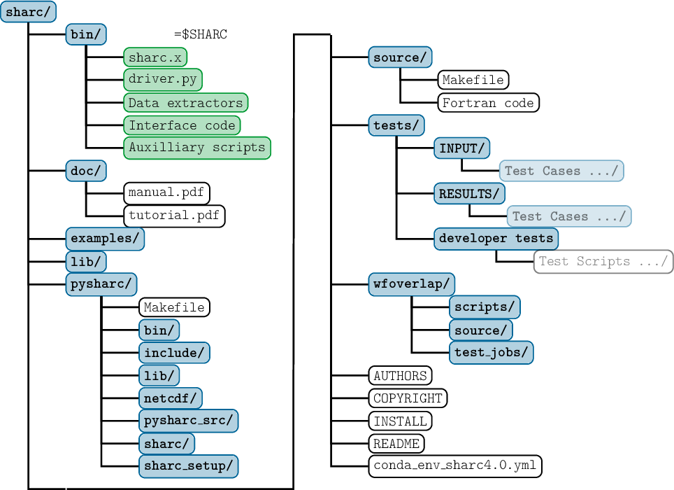
2.2.1 Libraries
Fortran installation
SHARC requires the BLAS, LAPACK and FFTW3 libraries. During the installation, it might be necessary to alter the LDFLAGS string in the Makefile, depending on where the relevant libraries are located on your system. In this way, it is for example possible to use vendor-provided libraries like the Intel MKL. For more details see the INSTALL file which is included in the SHARC distribution.
Python installation
In order to compile with pysharc, it is necessary to first create a suitable Python installation, which can be achieved with environment managers like (mini)conda or (micro)mamba. A working minimal environment can be created with (ignore the line break):
conda create -n sharc4.1 -c conda-forge python=3.12 numpy scipy h5py matplotlib
pyparsing netcdf4 gfortran_linux-64 pyscf openmm numba sympy pyyaml pytorch pytest ase
opt_einsum threadpoolctl pip joblib
Subsequently, the environment has to be activated with
conda activate sharc4.1
before one can proceed with the installation of SHARC.
Both commands also work with mamba instead of conda.
For a Python environment that is compatible with all currently known issues, use numpy=2.2 and scip=1.15.
The former avoids a known bug with RI-ECI and the latter avoids problems with executing parmed.
Instead of the command above, you should also be able to use
conda env create --file=$SHARC/../conda_env_sharc4.1.yml
You can also use the file $SHARC/../conda_env_sharc4.1.yml to install the compatible environment.
Note that these two approaches (copying the conda create line and using the yml files) might not produce 100% identical results.
Machine learning interfaces
To use the SPaiNN interface, clone the repository and install it:
git clone https://github.com/CompPhotoChem/SPaiNN.git
cd SPaiNN && pip install .
To use the SchNarc interface, install schnetpack 1, clone the repository, and install it:
pip install schnetpack==1.0.1
git clone https://github.com/schnarc/SchNarc.git
cd SchNarc && pip install .
Note that the SPaiNN and SchNarc interfaces are mutually exclusive, since they require different versions of SchNetPack!
Parmed
If you plan on using Amber and Ambertools to prepare and run QM/MM simulations with the OpenMM interface, it is useful to have the Python package parmed installed.
The script setup_from_prmtop.py depends on it.
Note that parmed is not compatible with recent versions of numpy.
Hence, it is recommended to create a separate Conda environment with parmed, numpy < 2.3, and scipy, to only run setup_from_prmtop.py.
Tequila
If you plan on using the Python package Tequila for quantum computing, it needs to be installed.
Thus, we recommend to install Tequila via
pip install tequila-basic
pip install qulacs
(see also https://github.com/tequilahub/tequila and https://github.com/tequilahub/tequila/releases).
Note that qulacs is one of the possible backends of tequila to run the quantum simulations.
Without installing it, tequila will fall back to a very slow symbolic backend, which leads to unacceptable performance.
Tequila also requires PySCF, but the conda environment described above will contain it.
Promdens
If you want to use the PDA excitation scheme via excite_with_promdens.py, you need to install the promdens Python package.
Currently, this is easiest available via pip install promdens.
PAWpySeed
In order to use the SHARC-VASP interface to compute overlaps, the pawpyseed Python/C package has to be correctly installed in the user’s conda environment.
Source code and documentation can be found at PAWpySeed.
To compile the underlying C code pawpyseed needs to be linked with MKL libraries. If these are not already present in the machine they can be installed in the Conda environment and added to the C compiler paths via
pip install mkl-devel
export C_INCLUDE_PATH=$CONDA_PREFIX/include:$C_INCLUDE_PATH
export LIBRARY_PATH=$CONDA_PREFIX/lib:$LIBRARY_PATH
export LD_LIBRARY_PATH=$CONDA_PREFIX/lib:$LD_LIBRARY_PATH
Subsequently, pawpyseed can be installed via
pip install cython
pip install pymatgen
pip install pawpyseed
In case of installation issues please check the official documentation for further details PAWpySeed.
Note also that you might need to set ulimit -s unlimited for VASP to run successfully.
2.2.2 Compilation of SHARC’s binaries
Compiling and installing (without pysharc)
To compile the Fortran90 programs of the SHARC suite, go to the source/ directory.
cd source/
and edit the Makefile by adjusting the variables in the top part.
If you only want to install regular SHARC (no pysharc or NetCDF), set USE_PYSHARC to false.
Then, inside source/ issuing the command:
make install
will compile the source, create all the binaries, and copy the binary files into the sharc/bin/ directory of the
SHARC distribution, which already contains all the python scripts which
come with SHARC.
Compiling and installing (with pysharc)
If you intend to perform computations with pysharc (using the efficient driver.py) or with NetCDF functionality, you need to set USE_PYSHARC to true in source/Makefile.
Note that currently, some options (adaptive time steps) are not supported in this way.
Due to a number of dependencies, compiling with pysharc is slightly more complicated than without.
The simplest way to compile both pysharc and the regular executables together is to
- run make install in pysharc/, then
- run make install in source/.
Environment setup
In order to use the SHARC suite, you have to set some environment variables. The recommended approach is to source either of the sharcvars files (generated by make) that are located in the bin/ directory. For example, if you have cloned SHARC into your home directory, just use:
source ~/sharc/bin/sharcvars.sh (for bourne shell users)
or
source ~/sharc/bin/sharcvars.csh (for c-shell type users)
Note that it may be convenient to put this line into your shell’s login
scripts.
2.2.3 WFOVERLAP Program
The SHARC package contains as a submodule the program WFOVERLAP, which is necessary for many functionalities of SHARC.
In order to install and test this program, see Section 6.35.
2.2.4 Test Suite
| Keyword | Description |
| $GAUSSIAN | Points to the main directory of the GAUSSIAN installation, which contains the GAUSSIAN executables (e.g., g09/g16 or l9999.exe). |
| $MNDO | |
| $MOLCAS | Points to the main directory of the OPENMOLCAS installation, containing molcas.rte and directories basis_library/ and bin/. |
| $MOPACPI | |
| $TURBOMOLE | Points to the main directory of the TURBOMOLE installation, which contains subdirectories like basen/, bin/, or scripts/. |
| $ORCA | Points to the directory containing the ORCA executables, e.g., orca, orca_gtoint, or orca_fragovl. |
| $NWCHEM | Points to the main installation directory, which contains subdirectories bin and data. |
| $VASP and $VASPHDF5 | Respectively point to the bin/ directory of the VASP installation, which contains the vasp_std,vasp_gam and vasp_ncl executables, and to the HDF5 installation folder used for the VASP compilation. Note that VASP should be compiled with HDF5 support. |
| $THEODORE | Points to the main directory of the THEODORE installation. $THEODORE/bin/ should contain analyze_tden.py. If you install and activate TheoDORE as usual, then $THEODIR is that folder. |
| $molcas | Should point to the same location as $MOLCAS, or another MOLCAS installation. Note that $molcas is only used by some COLUMBUS test jobs. Also note that $molcas does not need to point to the MOLCAS installation interfaced to COLUMBUS. |
| $orca | Should point to the same location as $ORCA, or another ORCA installation. Note that $orca is only used by some tests where ORCA is used as helper program (e.g., for setup_orca_opt.py or spin-orbit calculations with SHARC_TURBOMOLE.py). |
| $AMS | Points to the main directory of the ADF installation, which contains the file adfrc.sh and subdirectory bin/. |
| $BAGEL | Points to the main directory of the BAGEL installation, which contains subdirectories bin/ and lib/. |
| $COLUMBUS | Points to the directory containing the COLUMBUS executables, e.g., runls. |
| $MOLPRO | Points to the bin/ directory of the MOLPRO installation, which contains the molpro.exe file. |
After the installation, it is advisable to first execute the test suite of SHARC, which will test the fundamental functionality of SHARC to communicate with other programs.
Change to an empty directory and execute
$SHARC/tests.py
The interactive script will first verify the Python installation (no message will appear if the Python installation is fine).
Subsequently, the script prompts the user to enter which tests should be executed.
The script will also ask for a number of environment variables, which are listed in Table 2.1 if needed.
In SHARC4, the tests have been updated.
There is at least one test for each ab initio interface.
Additional tests are present for interfaces that require wfoverlap.x, TheoDORE, or interact somehow with other (optional) software.
In each case, the _curvature test (if present) tests the corresponding interface without any auxiliary programs.
All tests starting with the name of an ab initio program run short trajectories testing whether the main dynamics code, the interfaces, the quantum chemistry programs, and auxiliary programs (e.g., THEODORE, wfoverlap.x, ORCA) work correctly together.
If the installation was successful and Python is installed correctly, Analytical_overlap, LVC_overlap, and most tests named scripts_<NAME> should execute without error.
The test calculations involving the quantum chemistry programs can be used to check that SHARC can correctly call these programs and that they are installed correctly.
If any of the tests show differences between output and reference output, it is advisable to check the respective files (i.e., compare $SHARC/../tests/RESULTS/<job>/ to ./RUNNING_TESTS/<job>/).
Note that small differences (different sign of values or small numerical deviations) in the output can already occur when using a different version of the quantum chemistry programs, different compilers, different libraries, or different parallization schemes.
It should be noted that along trajectories, these small changes can add up to notably influence the trajectories, but across the ensemble these small changes will likely cancel out.
2.2.5 Additional Programs
For full functionality of the SHARC suite, several additional programs are recommended (all of these programs are currently freely available, except for some parts of AMBER):
- The Python package MATPLOTLIB.
If the MATPLOTLIB package, some auxiliary scripts (e.g., trajana_essdyn.py) can automatically generate certain plots.
- The GNUPLOT plotting software.
GNUPLOT is not strictly necessary, since all output files could be plotted using other plotting programs. However, a number of scripts from the SHARC suite automatically generate GNUPLOT scripts after data processing, allowing to quickly plot the results.
- A molecular visualization software able to read xyz files (e.g. MOLDEN, GABEDIT, MOLEKEL or VMD).
Molecular visualization software is needed in order to animate molecular motion in the dynamics.
- The THEODORE wave function analysis suite (version 3.0 or higher).
The wave function analysis package THEODORE allows to compute various descriptors of electronic wave functions (supported by some interfaces), which is helpful to follow the state characters along trajectories.
- The AMBER molecular dynamics package.
AMBER can be used to prepare topology files and initial conditions based on ground state molecular dynamics simulations (instead of using a Wigner distribution), which is especially useful for large systems.
- The ORCA ab initio package.
ORCA can be employed as external optimizer. In combination with the SHARC interfaces, it is possible to perform optimizations of minima, conical intersections, and crossing points for any method interfaced to SHARC.
- The FCCLASSES 3 package
FCCLASSES 3 can be used to compute vibronically resolved absorption/emission spectra from parametrized LVC models.
- The SHNITSEL–TOOLS package
SHNITSEL–TOOLS (Surface Hopping Nested Instances Training Set for Excited-state Learning) can be used to archive SHARC trajectories so that they can be contributed to the SHNITSEL–DATA repository.
2.2.6 Quantum Chemistry Programs
Even though SHARC comes with several interfaces for analytical potentials (and hence can be used without any quantum chemistry program), one of the main application of SHARC is certainly on-the-fly ab initio dynamics.
In this case, one of the following interfaced quantum chemistry programs is necessary:
- OpenMM
- GAUSSIAN (this release was checked against GAUSSIAN 16).
- ORCA (version 5.0 or 6.0).
- NWCHEM (version 7.2 or higher)
- TURBOMOLE (this release was checked against TURBOMOLE 7.8 and 7.9).
- OPENMOLCAS (this release was checked against OPENMOLCAS 24 and 25).
- MNDO (version 8.0 of 15 August 2019).
- MOPAC-PI (commit c2124b7a from 6 November 2024), including its internal version of TINKER.
- COLUMBUS 7
- COLUMBUS-MOLCAS interface for spin-orbit couplings.
- BAGEL (commit 0ea6b59 from Mar 27, 2019 or newer).
- AMSTERDAM DENSITY FUNCTIONAL (this release was tested against AMS 2024).
- MOLPRO (this release was checked against MOLPRO 2023).
- PYSCF with PySCF Forge
- TEQUILA (this release was checked against version 1.9.4).
- VASP (this release was tested against VASP 6.5.0 and 6.5.1).
See the relevant sections in Chapter 6 for a description of the quantum chemical methods available with each of these programs.
Chapter 3 Execution
The SHARC suite consists of the two main dynamics codes sharc.x and driver.py and a large set of auxiliary programs, like setup scripts and analysis tools.
Additionally, the suite comes with interfaces to several quantum chemistry software packages, as described elsewhere.
In the following, first it is explained how to run a single trajectory by setting up all necessary input for the dynamics code sharc.x manually, as a minimum working example.
Afterwards, the usage of the auxiliary scripts and the standard workflow is explained.
Detailed information on the SHARC input files is given in chapter 4.
Chapter 5 documents the different output files SHARC produces.
The interfaces are described in chapter 6 and the auxiliary scripts in chapter 7.
All relevant theoretical background is given in chapter 8.
More hands-on examples can be found in the Tutorial.
Additionally, we recommend several instructional videos recorded during the Cyber Training Workshop 2022 by Alexey Akimov from the University af Buffalo, NY.
These videos were recorded with SHARC3, but they still have instructional value for new users.
3.1 Running a single trajectory
3.1.1 Input files
Both drivers (sharc.x and driver.py) requires the same input files.
The most important file is called input and contains all settings for the dynamics.
The initial geometry is read from the geom file.
These two files are mandatory.
Additional, optional files can be used to provide the initial velocities (veloc), the initial state coefficients (coeff), and/or a laser field (laser).
Moreover, several files can be used to mask certain atoms from certain algorithms (atommask), to constrain certain bond lengths (rattle), to freeze the position of certain atoms (frozen),
and/or to define settings of the thermostat (thermostat_setting).
For all optional files; if not given, the missing information is automatically set according to some keywords in input.
The input files inside a trajectory folder are shown in Figure 3.1.
The content of the main input file is explained in detail in Section 4.1, the geometry file is specified in Section 4.2.
The specifications of the velocity, coefficient, and laser files are given in Sections 4.3, 4.4 and 4.5, respectively.
The atom mask file is likewise documented in Section 4.6, the RATTLE file in Section 4.7, the frozen atoms file in Section 4.8,
and the thermostat file in Section 4.9.
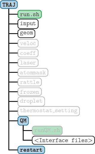
Additionally, the directory QM/ is required, containing the interface-specific input files.
If the trajectory is run with sharc.x, then the script QM/runQM.sh needs to be present, since the communication of sharc.x and the interfaces is implemented through this script.
Every time that sharc.x is making a quantum chemistry call, the current geometry and the requests are written to QM/QM.in.
Then, sharc.x calls QM/runQM.sh, waits for the script to finish and then reads the requested quantities from QM/QM.out.
The script QM/runQM.sh is fully responsible to generate the requested results from the provided input.
In virtually all cases, this task is handled by SHARC‘s interfaces (see Chapter 6), so that the script QM/runQM.sh has a particularly simple form:
cd QM/
$SHARC/SHARC_<NAME>.py QM.in
with the corresponding interface name given.
When running with sharc.x, this script is the location where the chosen interface is defined.
If the trajectory is instead run with driver.py, then the runQM.sh script does not need to be present.
The chosen interface is instead given to driver.py as a command line option.
Note that the interfaces in nearly all cases need additional input files, which must be present in QM/, independent of whether sharc.x or driver.py is used.
Most interfaces require two files, a template file and a reource file.
The contained information depends on the type of interface, but typically contains model information, quantum chemistry information, information about the child interfaces, and/or information about computational resources.
See Chapter 6 for details.
3.1.2 Running the dynamics code
Given the necessary input files, SHARC can be started by executing
user@host> $SHARC/sharc.x input
Note that besides the input file, at least the geometry file needs to be present (see chapter 4 for details).
If using the Python driver, the trajectory can be started by executing
user@host> $SHARC/driver.py -i <NAME> input
Note that for large systems (i.e., many electronic states and/or many atoms), it might in some cases be required to increase the stack size before starting either of the two dynamics drivers.
This can be achieved by
user@host> ulimit -s unlimited
If the system is too large and the stack size is not increased, typically SHARC will crash with a segmentation fault.
A running trajectory can be stopped gracefully after the current time step by creating an empty file STOP:
user@host> touch STOP
This is usually preferable to simply killing SHARC, because the current time step is properly finished and all files are correctly written for analysis and restart.
In order to restart a trajectory, add the restart keyword to the input file and call the driver again.
Please refer to Section 4.1 for further details.
In order to start a trajectory from time zero, no restart files from a previous run must be present, otherwise the dynamics drivers will raise an error.
A trajectory folder can conveniently be purged of most output files by using $SHARC/clean_traj.sh.
3.1.3 Output files
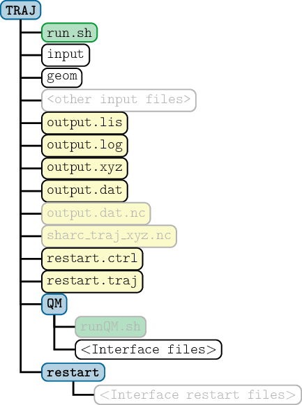
Figure 3.2 shows the content of a trajectory directory after the execution of either of SHARC‘s drivers.
There will be at least six new files.
The files that always will be created are output.log, output.lis, output.dat and output.xyz, as well as restart.ctrl and restart.traj.
Optionally, two more output files are created, output.dat.nc and output_NUC.dat.nc.
The file output.log contains mainly a listing of the chosen options and the resulting dynamics settings.
At higher print levels, the log file contains also information per time step (useful for debugging).
output.lis contains a table with one line per time step, giving active states, energies and expectation values.
output.xyz contains the geometries of all time steps (the comments to each geometry give the active state and current time).
output.dat contains a list of all important matrices and vectors at each time step.
This information can be extracted with data_extractor.x to yield plottable table files.
If netcdf output has been selected via the options in the input file, then output.dat.nc will be present as well.
If it is present, output.dat will only contain its header, but no information per time step.
The information per time step is contained in output.dat.nc.
Use data_extractor_NetCDF.x in this case.
If, the netcdf_separate_nuc option is chosen instead of regular netcdf output, then the output_NUC.dat.nc file is also present.
In this case, electronic information is in output.dat.nc and nuclear information in output_NUC.dat.nc, which is useful because one can separately control how often these files are written.
For details about the content of the output files, see chapter 5.
The restart files contain the full state of a trajectory and its control variables from the last successful time step.
These files are needed in order to restart a trajectory at this time step (either because the calculation failed, or in order to extend the simulation time beyond the original maximum simulation time).
The restart/ directory contains all persistent files that are needed for the interfaces (for restarting, but also between all time steps).
Usually, users do not need to inspect the restart files.
3.2 Typical workflow for an ensemble of trajectories
Usually, one is not interested in running only a single trajectory, since a single trajectory cannot reproduce the branching of a wave packet into different reaction channels.
In order to do so, within surface hopping an ensemble of independent trajectories is employed.
When dealing with a (possibly large) ensemble of trajectories, setup, management, and analysis need to be automatized.
Hence, the SHARC suite contains a number of scripts fulfilling different tasks in the usual workflow of setting up ensembles of trajectories.
The standard workflow is given schematically in Figure 3.3.
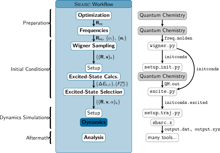
3.2.1 Initial condition generation
In the typical workflow, the user will first create a set of suitable initial conditions.
In the context of the SHARC package, an initial condition is a set of an initial geometry, initial velocity, initial occupied state, and initial wave function coefficients.
Many such sets are needed in order to setup physically sound dynamics simulations.
Generation of initial geometries and velocities
Within the SHARC suite, initial geometries and velocities can be generated based on a quantum harmonic oscillator Wigner distribution.
The theoretical background is given in Section 8.24.
The calculation is performed by wigner.py, which is explained in Section 7.1.
For special Wigner sampling tasks (e.g., only specific energies, modes), one can use wigner_state_selected.py (Section 7.2).
To combine the initial conditions of two molecules for collision/scattering simulations, one can use bimolecular_collision.py (Section 7.3).
As given in Figure 3.3, wigner.py needs as input the result of a frequency calculation in MOLDEN format.
The calculation can be performed by any quantum chemistry program and any method the user sees fit (there are some scripts which can aid in the frequency calculation and file conversion, see Sections 6.9.4, 6.10.4, 6.13.4,
6.15.4, 6.20.4, 6.23.6).
wigner.py produces the file initconds, which contains a list of initial conditions ready for further processing.
Alternatively, initial geometries and velocities can be extracted from molecular dynamics simulations in the ground state.
Currently, it is possible to either convert restart files from AMBER to an initconds file (using amber_to_initconds.py, see Section 7.4), convert a HFD5 file from a VASP MD simulation (using vasp_to_initconds.py, see Section 7.5), or to randomly sample snapshots from previous SHARC trajectories (using sharctraj_to_initconds.py, see Section 7.6).
In some cases, these tasks can also be performed with restartnc_to_xyz.py (Section 7.7) and sharctraj_to_xyz.py (Section 7.8).
Generation of initial coefficients and states
In the second preparation step, for each of the sampled initial geometries it has to be decided which excited state should be the initial one.
In most cases, this is done with excite.py (see Section 7.10).
In simple cases, the user can manually choose the initial excited state (optionally after diabatization).
Alternatively, the selection of initial states can be performed based on the excitation energies and oscillator strengths of the excited states at each initial geometry (this approximately simulates a delta-pulse excitation).
The latter options (diabatization or energies/oscillator strengths) make it necessary to carry out vertical excitation calculation before the selection of the initial states.
The calculations can be set up with setup_init.py (see Section 7.9).
This script prepares for each initial condition in the initconds file a directory with the necessary input to perform the calculation.
The user should then execute the run script (run.sh) in each of the directories (either manually or through a batch queueing system).
After the vertical excitation calculations are completed, the vertical excitation energies and oscillator strengths of each calculation are collected by excite.py (see 7.10).
The same script then performs the selection of the initial electronic state for each initial geometry.
The results are written to a new file, initconds.excited.
This file contains all information needed to setup the ensemble.
Additionally, spectrum.py (7.11) can calculate absorption spectra based on the initconds.excited file.
This may be useful to verify that the level of theory chosen is appropriate (e.g., by comparing to an experimental spectrum), or to choose a suitable excitation window for the determination of the initial state.
Since SHARC 4.1, initial electronic states can also be determined by the electron-only explicit (EOE) excitation scheme [46].
Here, for each initial condition a short SHARC simulation with frozen nuclei (using SHARC_QMOUT.py is run under the influence of a laser pulse.
The obtained electronic populations are used to stochastically select the initial active state for the actual dynamics simulations.
Additionally, this scheme determines for each selected initial state a starting time, which is stored in the initconds file.
The EOE excitation scheme is run using the scripts setup_laser_excitation.py (Section 7.13) and excite_laser_excitation.py (Section 7.14).
Also since SHARC 4.1, initial electronic states can also be determined by the promoted density approach (PDA) [47].
This scheme is a significant improvement over the vertical excitation scheme of excite.py.
It includes the Wigner distribution of a user-defined laser pulse in the computation of the selection probabilities.
This scheme also determines for each selected initial state a starting time, which is stored in the initconds file.
The PDA scheme can be run with the promdens code of the original authors, using the wrapper excite_with_promdens.py (7.15).
Currently, there is no automatic setup to prepare specific initial electronic coefficients beyond what the driver automatically set based on the state and coeff keywords.
3.2.2 Setting up the dynamics simulations
To prepare for the trajectory setup, in some cases specific input files need to be prepared.
This includes laser files that can be produced with laser.x (Section 7.12) or QM/MM-related files that can be created with setup_from_prmtop.py (Section 7.16).
Further interface-specific files can be produced with, e.g., molcas_input.py (Section 6.15.4),
molpro_input.py (Section 6.23.6),
as well as setup_LVCparam.py,
create_LVCparam.py,
and modify_LVC_template.py (see all three in Section 6.4.4).
The memory consumption of RESP fits can be estimated, too (see Section 7.17).
However, for many interface, one only needs to take an example template file from $SHARC/../examples/ and adapt it to the specific needs.
Based on the initial conditions given in initconds.excited and the prepared input/template files, the input for all trajectories in the ensemble can be setup by setup_traj.py (see Section 7.18).
The script produces one directory for each trajectory, containing the input files for the dynamics drivers and the selected interface.
3.2.3 Running the dynamics simulations
In order to run a particular trajectory, the user should execute the run script (run.sh) in the directory of the trajectory.
Since those calculations can run between minutes and several weeks (depending on the level of theory used and the number of time steps), it is advisable to submit the run scripts to a batch queueing system.
The progress of the simulations can be monitored most conveniently in the output.lis files.
If the calculations are running in some temporary directory, the output files can be copied to the local directory (where they were setup) with the scp wrapper retrieve.sh (see Section 7.19).
This allows to perform ensemble analysis while the trajectories are still running.
If a trajectory fails, the temporary directory where the calculation is running is not deleted.
The file README will be created in the trajectory’s directory, giving the time of the failure and the location of the temporary data, so that the case can be investigated.
In order to signal SHARC to terminate a trajectory after the current time step is completed, the user can create a (possibly empty) file STOP in the working directory of the trajectory (the directory where sharc.x is running).
To remove all output files of a trajectory and restore it to the status after setup, one can use clean_traj.sh (Section 7.20).
The status of the ensemble of trajectories can be checked with diagnostics.py (Section 7.21).
This script checks the presence and integrity of all relevant files, the progress of all trajectories, and warns if trajectories behave unexpectedly (non-conversion of total energy, intruder states, etc).
3.2.4 Analysis of the dynamics results
Each trajectory can be analyzed independently by inspecting the output files (see chapter 5).
Most importantly, calling data_extractor.x (7.22) or data_extractor_NetCDF.x (7.23) on the output.dat file of a trajectory creates a number of formatted files.
If needed, the output.dat and output.dat.nc files can be interconverted with data_converter.x (7.24) and data_converter_to_ASCII.x (7.25).
In special cases, the file output_NUC.dat.nc is produced, which can be converted to output.xyz with data_extractor_NUC_xyz.py (Section 7.26).
The files produced by the extractor programs can be plotted with the help of make_gnuscript.py (Section 7.27) and GNUPLOT.
The nuclear geometries in output.xyz file can be analyzed in terms of internal coordinates (bond lengths, angles, ring conformations, etc.) using geo.py (Section 7.28) and in terms of normal mode coordinates using geo_NM.py (Section 7.29).
The manual analysis of all individual trajectories is usually a good idea to verify that the trajectories are correctly executing, and to find general reaction pathways.
The manual analysis often permits to formulate some hypotheses, which can then be verified with the statistical analysis tools.
For the statistical analysis of the complete ensemble, the first step should usually be to run diagnostics.py (Section 7.21).
This script will determine how long the different trajectories are, and, more importantly, will check the trajectories for file integrity, conservation of total energy, and continuity of potential/kinetic energy.
Based on a set of customizable criteria, the script determines for each trajectory a “maximum usable time”.
The script then can mark all trajectories with maximum usable time below a given threshold to be excluded from analysis (by creating a file DONT_ANALYZE in the trajectory’s directory).
The other analysis scripts will then ignore trajectories marked by diagnostics.py.
Trajectories can also be manually excluded from analysis, by creating a file called CRASHED, DEAD, or RUNNING in the respective directory.
After the trajectories were checked and unsuitable ones excluded, the statistical analysis scripts can be used.
The script populations.py (Section 7.31) can calculate average excited-state populations using different algorithms and prepares files needed to obtain time constants and their uncertainties.
The script transition.py (Section 7.32) can analyze the total number of hops between all pairs of states in an ensemble, allowing to identify relevant relaxation routes in the dynamics.
Using the script make_fit.py (Section 7.33), it is possible to make elaborate global fits of chemical kinetics models to the populations data, allowing to extract rate constants from the populations, and to compute errors for these rate constants.
The script crossing.py (Section 7.34) can find and extract notable geometries, e.g., those geometries where a surface hop between two particular states occurred.
Using trajana_essdyn.py (Section 7.35) it is possible to perform essential dynamics analysis.
Finally, data_collector.py (Section 7.36) can merge arbitrary tabulated data from the trajectories and perform various analysis procedures (compute mean/standard deviation, data convolution, summation, integration), which can be used to compute, e.g., time-dependent distribution functions or time-dependent spectra.
Furthermore, the script delay_time.py (Section 7.37) computes time correlation distributions for arbitrary, threshold-detected events, e.g., the distribution of times it takes a molecule to dissociate after a particular surface hop.
Three new analysis scripts in SHARC4 can be used to collect coordinate data for each time step, align them in specific ways, and compute one- and three-dimensional distribution functions.
These scripts are align_and_reorder_traj.py (Section 7.38), frames_to_RDF.py (Section 7.39), and frames_to_dx.py (Section 7.40).
As they are intended for large-scale analysis of big systems, they are only compatible with NetCDF output.
The output of frames_to_RDF.py can be used to compute X-ray scattering signals using RDF_to_scattering.py (Section 7.41).
The scripts frames_to_RDF.py and RDF_to_scattering.py produce one file for each time step; these files can be merged into one total file using data_merger.py (Section 7.42).
If the trajectories were set up with the EOE or PDA excitation schemes, each trajectory has a starting time (the point in time where the excitation happened), which is stored in a start.time file in each trajectory folder.
This file is automatically recognized by population.py, geo.py, geo_NM.py, data_extractor.x, and data_extractor_NetCDF.x when they write out results.
Each trajectory will thus be shifted in time and start at a slightly different point in time.
The output.lis file can also be shifted in time with shift_output_lis.py (Section 7.30).
3.3 Programs and Scripts of the SHARC Suite
The following tables list all the programs in the SHARC suite.
The rightmost column gives the section where the program is documented.
3.3.1 Setup and Preparation
| wigner.py | Creates initial conditions from a Wigner distribution. | 7.1 |
| wigner_state_selected.py | Creates initial conditions from selected vibrational states. | 7.2 |
| bimolecular_collision.py | Creates initial conditions from two initconds files. | 7.3 |
| amber_to_initconds.py | Creates initial conditions from Amber restart files. | 7.4 |
| vasp_to_initconds.py | Creates initial conditions from VASP molecular dynamics trajectories. | 7.5 |
| sharctraj_to_initconds.py | Creates initial conditions from SHARC trajectories. | 7.6 |
| restartnc_to_xyz.py | Directly creates QM.in or geom/veloc files from Amber restart files. | 7.7 |
| sharctraj_to_xyz.py | Directly creates QM.in or geom/veloc files from SHARC trajectories. | 7.8 |
| setup_init.py | Sets up initial vertical excitation calculations. | 7.9 |
| excite.py | Generates excited state lists for initial conditions and selects initial states. | 7.10 |
| spectrum.py | Generates absorption spectra from initial conditions files. | 7.11 |
| laser.x | Prepares files containing laser fields. | 7.12 |
| setup_laser_excitation.py | Set up electron-only simulations with SHARC_QMOUT.py | 7.13 |
| excite_laser_excitation.py | Selects initial states and start times from electron-only simulations. | 7.14 |
| excite_with_promdens.py | Selects initial states and start times with the PDA scheme. | 7.15 |
| setup_from_prmtop.py | Sets up files for QM/MM simulations (topology/force field files, RATTLE files, and QM/MM table files) from Amber topology files. | 7.16 |
| setup_traj.py | Sets up the dynamics simulations based on the initial conditions. | 7.18 |
| setup_LVCparam.py | Sets up single point calculations for LVC parametrization. | 6.4.4 |
| create_LVCparam.py | Produces LVC model files from parametrization data. | 6.4.4 |
| modify_LVC_template.py | Removes states, modes, or dipole moments from LVC parameter files. | 6.4.4 |
| GAUSSIAN_freq.py | Converts GAUSSIAN output files of frequency calculations to Molden format. | 6.9.4 |
| ORCA_hess_freq.py | Converts ORCA Hessian files to Molden format. | 6.10.4 |
| vasp_to_molden.py | Converts VASP output files of phonon calculations to Molden format. | 6.13.4 |
| AMS_ADF_freq.py | Converts ADF output files of frequency calculations to Molden format. | 6.20.4 |
| molcas_input.py | Prepares MOLCAS input files and template files for the MOLCAS interface. | 6.15.4 |
| molpro_input.py | Prepares MOLPRO input files and template files for the MOLPRO interface. | 6.23.6 |
3.3.2 Trajectory Running and Management
| sharc.x | Legacy dynamics driver with full feature support but slow I/O-based interface communication. | 3.4.1 |
| driver.py | New PySHARC dynamics driver with fast in-memory interface communication but with a few unsupported features. | 3.4.2 |
| retrieve.sh | scp wrapper to retrieve dynamics output during the simulation. | 7.19 |
| clean_traj.sh | Removes all output and restart files from a trajectory. | 7.20 |
| diagnostics.py | Checks ensembles for integrity, progress, energy conservation. | 7.21 |
3.3.3 Analysis
| data_extractor.x | Extracts plottable results from the SHARC output data file. | 7.22 |
| data_extractor_NetCDF.x | Extracts plottable results from the SHARC output data file in NetCDF format. | 7.23 |
| data_converter.x | Converts output.dat files to output.dat.nc files. | 7.24 |
| data_converter_to_ASCII.x | Converts output.dat.nc files to output.dat.cp. | 7.25 |
| data_extractor_NUC_xyz.py | Converts output_NUC.dat.nc files to output.xyz | 7.26 |
| make_gnuscript.py | Creates gnuplot scripts to plot trajectory data. | 7.27 |
| geo.py | Calculates internal coordinates from xyz files. | 7.28 |
| geo_NM.py | Calculates normal model coordinates from xyz files. | 7.29 |
| shift_output_lis.py | Applies the excitation time shift to the output.lis file. | 7.30 |
| populations.py | Calculates ensemble populations. | 7.31 |
| transition.py | Calculates total number of hops within an ensemble. | 7.32 |
| make_fit.py | Performs kinetic model fits and bootstrapping. | 7.33 |
| crossing.py | Extracts specific geometries from ensembles. | 7.34 |
| trajana_essdyn.py | Performs an essential dynamics analysis for an ensemble. | 7.35 |
| data_collector.py | Collects data from tabular files and performs various analyses. | 7.36 |
| delay_time.py | Collects delay time distributions between threshold-detected events. | 7.37 |
| align_and_reorder_traj.py | Collects, aligns, and converts coordinates into NetCDF files per time step. | 7.38 |
| frames_to_RDF.py | Computes radial histograms/distribution functions from NetCDF files. | 7.39 |
| frames_to_dx.py | Computes 3D distributions in dx format from NetCDF files. | 7.40 |
| RDF_to_scattering.py | Computes X-ray scattering from histogram data. | 7.41 |
| data_merger.py | Merges output files from frames_to_RDF.py and RDF_to_scattering.py into one single file. | 7.42 |
3.3.4 Others
| tests.py | Script to automatically run the SHARC test suite. | 2.2.4 |
| wfoverlap.x | Program to compute wave function overlaps, used by most interfaces. | 6.35 |
| Orca_External | Script to carry out optimizations with ORCA4 as optimizer and SHARC as gradient provider. | 7.43 |
| otool_external | Script to carry out optimizations with ORCA5/6 as optimizer and SHARC as gradient provider. | 7.43 |
| setup_orca_opt.py | Script to setup optimizations with ORCA as optimizer and SHARC as gradient provider. | 7.43 |
| setup_single_point.py | Script to setup single point calculations with SHARC interfaces. | 7.44 |
| QMout_print.py | Script to convert a QM.out file to a table with energies and oscillator strengths. | 7.45 |
| FCClasses_from_LVC.py | Prepare input for FCclasses from LVC parameter files. | 6.4.5 |
| resp_memory_estimator.py | Script to compute memory usage of RESP fits based on an xyz file and a PySCF basis set. | 7.17 |
3.3.5 Interfaces
Stub interfaces
| SHARC_DO_NOTHING.py | Provides zeros for all requested quantities (overlap matrices are returned as unit matrices). Intended for testing purposes only. | 6.1 |
| SHARC_QMOUT.py | Provides the Hamiltonian (with SOCs) and dipole moments from a provided QM.out file and returns zeros otherwise (unit matrix overlaps). Intended for SHARC trajectories with frozen nuclei/electron-only dynamics (e.g., via setup_laser_excitation.py, Section 7.13). | 6.2 |
Fast interfaces
| SHARC_ANALYTICAL.py | Provides SOCs, gradients, overlaps, dipole moments, and dipole moment derivatives based on analytical expressions formulated in sympy of diabatic matrix elements defined in Cartesian coordinates. | 6.3 |
| SHARC_LVC.py | Provides SOCs, gradients, nonadiabatic couplings, overlaps, and dipole moments based on linear/quadratic-vibronic coupling models defined in mass-weighted normal mode coordinates. | 6.4 |
| SHARC_SPAINN.py | Calculates gradients, dipole moments, and nonadiabatic coupling vectors using SPaiNN machine learning models. | 6.5 |
| SHARC_SCHNARC.py | Provides gradients, dipole moments, and nonadiabatic coupling vectors using (Field)Schnet machine learning models. Can do electrostatic embedding. | 6.6 |
| SHARC_OPENMM.py | Provides gradients, dipole moments, and multipolar fits using OpenMM and Amber force fields. | 6.7 |
Ab initio interfaces
| SHARC_GAUSSIAN.py | Provides dipole moments, gradients, overlaps, Dyson norms, TheoDORE wave function descriptors, multipolar fits, and density matrices at the TD-DFT level of theory using GAUSSIAN. Can do electrostatic embedding. | 6.9 |
| SHARC_ORCA.py | Provides SOCs, dipole moments, gradients, overlaps, Dyson norms, and TheoDORE wave function descriptors at the TD-DFT level of theory using ORCA. Can do electrostatic embedding. | 6.10 |
| SHARC_BASICORCA.py | Provides dipole moments and gradients at the TD-DFT level of theory using ORCA | 6.11 |
| SHARC_NWCHEM.py | Provides dipole moments, gradients, and overlaps at the TD-DFT level of theory using NWCHEM. | 6.12 |
| SHARC_VASP.py | Provides /ground-state) gradients, overlaps and (null) dipole moments at the KS-TD-DFT level using VASP. | 6.13 |
| SHARC_TURBOMOLE.py | Provides SOCs, dipole moments, gradients, overlaps, Dyson norms, and TheoDORE wave function descriptors at the ADC(2) and CC2 levels of theory using TURBOMOLE. Can do electrostatic embedding. Some restrictions apply to CC2. Needs ORCA for SOCs. | 6.14 |
| SHARC_MOLCAS.py | Provides SOCs, dipole moments, gradients, nonadiabatic coupling vectors, overlaps, Dyson norms, TheoDORE wave function descriptors, multipolar fits, and density matrices for CASSCF/RASSCF, several CASPT2 variants, and some PDFT variants (using OPENMOLCAS). Can do electrostatic embedding. | 6.15 |
| SHARC_MNDO.py | Provides dipole moments, gradients, nonadiabatic coupling vectors, and overlaps at the semiempirical MRCI level of theory using the MNDO code. Restricted to singlet states. Can do electrostatic embedding. | 6.16 |
| SHARC_MOPACPI.py | Provides dipole moments, gradients, nonadiabatic coupling vectors, and overlaps at the semiempirical MRCI level of theory using the MOPAC-PI code. Restricted to singlet states. Has built-in QM/MM capabilities. | 6.17 |
| SHARC_TEQUILA.py | Provides dipole moments, gradients, nonadiabatic coupling vectors, and overlaps based on variational quantum eigensolver computations using different ansätze. Restricted to singlet states. | 6.18 |
| SHARC_LEGACY.py | Provides SOCs, dipole moments, gradients, nonadiabatic coupling vectors, overlaps, Dyson norms, and TheoDORE wave function descriptors by calling any of the legacy interfaces below. | 6.19 |
Legacy ab initio interfaces
| SHARC_AMS_ADF.py | Provides SOCs, dipole moments, gradients, overlaps, Dyson norms, and TheoDORE wave function descriptors at the TD-DFT level of theory using ADF. | 6.20 |
| SHARC_COLUMBUS.py | Provides SOCs, dipole moments, gradients, nonadiabatic couplings, overlaps, and Dyson norms at the CASSCF, RASSCF, and MRCISD levels of theory using COLUMBUS. Some restrictions apply depending on the chosen integral engine. |
6.21 |
| SHARC_BAGEL.py | Provides dipole moments, gradients, nonadiabatic couplings, and overlaps at the CASSCF, CASPT2, MS-CASPT2, and XMS-CASPT2 level of theory using BAGEL. Restricted to singlet states. | 6.22 |
| SHARC_MOLPRO.py | Provides SOCs, dipole moments, gradients, nonadiabatic couplings, overlaps, and Dyson norms at the CASSCF level of theory (using MOLPRO). | 6.23 |
| SHARC_PYSCF.py | Provides dipole moments, gradients, and nonadiabatic couplings at the CASSCF, MC-PDFT, CMS-PDFT, and L-PDFT levels of theory (using PYSCF). Restricted to singlet states. | 6.24 |
Single-child hybrid interfaces
| SHARC_ASE_DB.py | Provides any requested data from a single child interface. Stores geometry, point charges, and all results in a database using the ASE package. | 6.25 |
| SHARC_UMBRELLA.py | Provides any requested data from a single child interface. Adds harmonic restraints to energies and gradients, using various collective variables. | 6.26 |
| SHARC_DROPLET.py | Provides any requested data from a single child interface. Adds harmonic positional restraints to energy and gradients. | 6.27 |
| SHARC_CPA.py | Provides any requested data from the child interface, but replaces any gradient request by a request for the ground state gradient only. It returns the groudn state gradient as gradient of all states. | 6.28 |
| SHARC_NUMDIFF.py | Provides requested data from a single child interface. Also provides gradients, nonadiabatic couplings, and dipole moment/SOC derivatives from finite differences. | 6.29 |
Multi-child hybrid interfaces
| SHARC_QMMM.py | Provides requested data by performing an electrostatic embedding QM/MM calculation with one QM and two MM children. | 6.30 |
| SHARC_ECI.py | Provides energies and dipole moments by performing an excitonic configuration interaction calculation based on several fragments computed with child interfaces. Requires electronstatic embedding, multipolar fitting, and density matrices from all children. | 6.31 |
| SHARC_ADAPTIVE.py | Provides requested data from several child interfaces with a quorum-based termination criterion. | 6.32 |
| SHARC_FALLBACK.py | Provides requested data from a trial child. If the trial child fails, provides data from a backup child instead. | 6.33 |
3.4 The SHARC dynamics drivers
The original dynamics driver of SHARC, present since version 1.0, is sharc.x.
This is a monolithic Fortran program that performs all steps of the SHARC method, including input parsing, initialization, nuclear propagation, requesting electronic structure information from an interface, electronic propagation, computing hopping probabilities, making hopping decisions, and producing output.
The communication with the electronic structure interfaces is based on writing and reading ASCII files, as described in Section 6.34.
Besides the reading and writing of several files (which takes time and limits precision), this form of communication also implies that the electronic structure interface is restarted/reloaded into memory at every time step (or even several times per time step).
Hence, this is a relatively slow form of communication, which typically adds a few tenths of a second up to a few seconds per time step.
For expensive on-the-fly quantum chemistry interfaces, where each time step takes at least several minutes, this time overhead is negligible.
However, for very fast potential energy surface methods (like analytical models, vibronic coupling models, machine learning models, or force fields), the overhead might well take much longer than the actual computation.
To overcome the limitations of file I/O and reloading interface code, with SHARC2.1 the PySHARC approach was introduced.
PYSHARC is an implementation of the SHARC dynamics driver in Python that directly calls the Fortran routines of sharc.x through the Python-C API via intermediate C routines.
In this way, both the Fortran code and the interface code can be run within the same program, omitting file-based communication and reloading of interface code.
Using PySHARC can reduce the cost per time step for the mentioned fast methods from few seconds to few milliseconds, providing a dramatic speedup of the SHARC simulations.
Consequently, the use of PySHARC is highly advisable for SHARC simulations with all fast interfaces.
Whereas in SHARC3, each interface required a separate PySHARC driver, in SHARC4, all interfaces use the common driver.py.
PySHARC is intended to change the SHARC workflow as little as possible.
Basically all features of sharc.x are supported.
The only change that needs to be applied is to call the pysharc driver instead of sharc.x.
The general trajectory setup script setup_traj.py can create input files for either driver.
The high efficiency of PySHARC is optimally combined with an efficient way of producing output.
As the historical output format of SHARC in terms of ASCII files is not optimized for performance, during the implementation of PySHARC also new output routines, using the NetCDF binary file format, were implemented.
It is advisable that every time PySHARC is run, output is written in NetCDF format.
Details of NetCDF output are documented in Section 5.4.
As described in Section 2.2, the SHARC code can be compiled in two ways, without and with PySHARC support.
If compiled without PySHARC support, then only sharc.x is available.
If compiled with PySHARC support, then both drivers will be created.
It is noteworthy that the sharc.x with PySHARC is compiled differently and supports some different options than if compiled without PySHARC support.
3.4.1 Original driver: sharc.x
The sharc.x driver is executed with
user@host> $SHARC/sharc.x <filename>
Typically, the input file name is input.
Instead of the file name, one can provide any one of the arguments -v, -version, or -info.
In this way, sharc.x will print its version infos and then exits.
When using sharc.x, the verbosity of the driver code is controlled by the printlevel keyword in the input file.
The verbosity of the employed interfaces can be controlled via the environment variables $SHARCLOG or $SHARC_LOG.
Possible settings are 40 for ßilent”, 11 for default verbosity, and 10 for “debug” print.
Within sharc.x, if the package was compiled without PySHARC support, the no support for NetCDF output is provided.
The only output_format is ascii.
However, if the package was compiled without PySHARC, then the Bulirsch-Stoer-Hack and adaptive velocity Verlet nuclear integrators are available.
3.4.2 PySHARC driver: driver.py
The PySHARC driver can be execited with
user@host> $SHARC/driver.py -i <NAME> <filename> [options]
Here, <filename> has the same meaning as for sharc.x.
The -i option (alias -interface) is used to select the interface that is employed in the dynamics.
If hybrid interfaces are used, the - option only specifies the top-level interface; its child interfaces are set in the input files for the top-level interface, and driver.py does not know about the child interfaces.
By default, driver.py initializes its child interface in the so-called persistent mode.
This mode only has an effect for fast interfaces (those derived from SHARC_FAST.py); most other interfaces simply ignore this mode.
In persistent mode, fast interfaces will not write interface-specific restart files in each time step, but only in the very last time step.
This improves performance with those interfaces, but leaves the output without restart files in the case of a crash/external termination.
Using -p or -nonpersistent, the driver can be ordered to initialize the interface in non-persistent mode, where restart files are written every time step.
Since SHARC 4.1, the driver also offers the option to choose either the fast queue (indicating to hybrid interfaces to use a light-weight queue for their children) or the full subprocess queue (indicating to hybrid interfaces to use a resource-aware queue with true subprocesses).
The fast queue is recommended for fast children, while the full queue is recommended for ab initio children.
To choose the fast queue, use the -fast_queue option.
The full queue is the default behaviour.
With driver.py, the verbosity of the used interface(s) can be directly controlled via command line options.
Using -s or -silent, only minimal information is printed.
The level -s or -verbose provides the standard amount of output.
Using -d or -debug, additional information on the execution of the interfaces is provided.
Instead of using these flags, the environment variables $SHARCLOG or $SHARC_LOG can be used.
Note that the flags and environment variables have no effect on the verbosity of the dynamics code itself.
When the package is compiled with PySHARC support, then via driver.py (and also via sharc.x), NetCDF output might be available (needs to be separately activated during compilation).
In turn, with PySHARC support, the Bulirsch-Stoer-Hack and adaptive velocity Verlet integrators are not available.
Other options that in SHARC3 were not supported by PySHARC are now available in SHARC4.
Chapter 4 Input files
In this chapter, the format of all SHARC input files are presented. Those are the main input file (here called input), the geometry file, the velocity file, the coefficients file, the laser file, and the atom mask file. Only the first two are mandatory, the others are optional input files. All input files are ASCII text files.
4.1 Main input file
This section presents the format and all input keywords for the main SHARC input. Note that when using setup_traj.py, full knowledge of the SHARC input keywords is not required.
4.1.1 General remarks
The input file has a relatively flexible structure. With very few exceptions, each single line is independent. An input line starts with a keyword, followed optionally by a number of arguments to this keyword. Example:
stepsize 0.5
Here, stepsize is the keyword, referring to the size of the time steps for the nuclear motion in the dynamics. 0.5 gives the size of this time step, in this example 0.5 fs.
A number of keywords have no arguments and act as simple switches (e.g., restart, gradcorrect, grad_select, nac_select, ionization, track_phase, dipole_gradient). Those keywords can be prefixed with no to explicitly deactivate the option (e.g., norestart deactivates restarts).
In each line a trailing comment can be added in the input file, by using the special character #. Everything after # is ignored by the input parser of SHARC. The input file also can contain arbitrary blank lines and lines containing only comments. All input is case-insensitive.
The input file is read by SHARC by subsequently searching the file for all known keywords. Hence, unknown or misspelled keywords are ignored. Also, the order of the keywords is completely arbitray. Note however, that if a keyword is repeated in the input only the first instance is used by the program.
4.1.2 Input keywords
In Table 4.1, all input keywords for the SHARC input file are listed.
|
Table 4.1: Input keywords for sharc.x and driver.py. The first column gives the name of the keyword, the second lists possible arguments and the third line provides an explanation. Defaults are marked like this. $n denotes the n-th argument to the keyword.
|
|||
| Keyword | Arguments | Explanation | |
| printlevel | integer | Controls the verbosity of the log file. | |
| $1=0 | Log file is empty | ||
| $1=1 | + List of internal steps | ||
| $1=2 | + Input parsing information | ||
| $1=3 | + Some information per time step | ||
| $1=4 | + More information per time step | ||
| $1=5 | + Much more information per time step | ||
| restart | Dynamics is resumed from restart files. | ||
| norestart | Dynamics is initialized from input files. This gives an error if restart files are present. | ||
| norestart takes precedence. | |||
| write_restart_files | Write restart files. | ||
| nowrite_restart_files | Don’t write restart files. Restart will not be possible! | ||
| write_restart_files takes precedence. | |||
| retain_restart_files | integer | Retain interface restart files for the last $1 steps. | |
| $=2 or 3 | With overlaps, default is 3 and minimum value is 1. | ||
| rngseed | integer | Seed for the random number generator. | |
| 10997279 | Used for surface hopping and AFSSH decoherence. | ||
| compatibility | $1=0 | Compatibility mode disabled. | |
| $1=1 | Do not draw a second random number per step (for decoherence). | ||
| – Input file keywords – | |||
| geomfile | quoted string | File name containing the initial geometry. | |
| “geom” | |||
| velocfile | quoted string | File containing the initial velocities. | |
| “veloc” | Only read if veloc external. | ||
| coefffile | quoted string | File containing the initial wave function coefficients. | |
| “coeff” | Only read if coeff external. | ||
| laserfile | quoted string | File containing the laser field. | |
| “laser” | Only read if laser external. | ||
| atommaskfile | quoted string | File containing the atom mask. | |
| “atommask” | Only read if atommask external. | ||
| rattlefile | quoted string | File containing the list of bond length constraints. | |
| “rattle” | Only read if rattle. | ||
| – Trajectory initialization keywords – | |||
| veloc | string | Sets the initial velocities. | |
| $1=zero | Initial velocities are zero. | ||
| $1=random $2 float | Random initial velocities with $2 eV kinetic energy per atom. | ||
| $1=external | Initial velocities are read from file. | ||
| nstates | list of integers | Number of states per multiplicity. | |
| $1 (1) | Number of singlet states | ||
| $2 (0) | Number of doublet states | ||
| $3 (0) | Number of triplet states | ||
| $… (0) | Number of states of higher multiplicities | ||
| charge | list of integers | Charge of states per multiplicity. | |
| $1 (no default) | Charge of singlet states | ||
| $2 | Charge of doublet states | ||
| $3 | Charge of triplet states | ||
| $… | Charge of states of higher multiplicities | ||
| actstates | list of integers | Number of active states per multiplicity. | |
| same as nstates | By default, all states are active. | ||
| state | integer, string | Specifies the initial state. | |
| (no default; SHARC exits if state is missing). | |||
| $1 | Initial state. | ||
| $2=MCH | Initial state and coefficients are given in MCH representation. | ||
| $2=diag | Initial state and coefficients are given in diagonal representation. | ||
| coeff | string | Sets the wave function coefficients. | |
| $1=auto | Initial coefficient are determined automatically from initial state. | ||
| $1=external | Initial coefficients are read from file. | ||
| – Laser field keywords – | |||
| laser | string | Sets the laser field. | |
| $1=none | No laser field is applied. | ||
| $1=internal | Laser field is calculated at each time step from internal function. | ||
| $1=external | Laser field for each time step is read during initialization. | ||
| laserwidth | float | Laser bandwidth used to detect induced hops. | |
| 1.0 eV | |||
| – Time step keywords – | |||
| stepsize | float | Length of the nuclear dynamics time steps in fs. | |
| 0.5 fs | |||
| nsubsteps | integer | Number of substeps for the integration of the electronic equation of motion. | |
| 25 | |||
| nsteps | integer | Number of simulation steps. | |
| 3 | |||
| tmax | float | Total length of the simulation in fs. | |
| No effect if nsteps is present. | |||
| killafter | float | Terminates the trajectory after $1 fs in the lowest state. | |
| -1 | If $1 < 0, trajectories are never killed. | ||
| – Integrator keywords – | |||
| integrator | string | Method to control the integrator. | |
| $1=fvv | Fixed time step velocity Verlet integrator. | ||
| $1=avv | Adaptive time step velocity Verlet integrator (not in pysharc). | ||
| convthre | float | Convergence threshold for adaptive integrators (in eV). | |
| $1=1e-04 | |||
| stepsize_min | float | Minimum step size allowed in adaptive velocity Verlet. | |
| $1=stepsize/16 | |||
| stepsize_max | float | Maximum step size allowed in adaptive velocity Verlet. | |
| $1=stepsize*2 | |||
| stepsize_min_exp | integer | Minimum power of 2 allowed in adjusting the time step in adaptive velocity Verlet. If used, this keyword will overwrite keyword stepsize_min. | |
| $1=-4 | |||
| stepsize_max_exp | integer | Maximum power of 2 allowed in adjusting the time step in adaptive velocity Verlet. If used, this keyword will overwrite keyword stepsize_max. | |
| $1=2 | |||
| – Dynamics setting keywords that applicable to both TSH and SCP methods – | |||
| method | string | Nonadiabatic dynamics method. | |
| $1=tsh | Uses trajectory surface hopping. | ||
| $1=scp, ehrenfest | Uses self-consistent potential methods. | ||
| coupling | string | Quantities describing the nonadiabatic couplings. | |
| $1=ddr,nacdr | Uses vectorial nonadiabatic couplings 〈ψα|∂/∂R|ψβ〉. | ||
| $1=ddt,nacdt | Uses temporal nonadiabatic couplings 〈ψα|∂/∂t|ψβ〉. | ||
| $1=overlap | Uses the overlaps 〈ψα(t0)|ψβ(t)〉 (local diabatization). | ||
| $1=ktdc | Uses curvature driven approximation for time derivative coupling. | ||
| ktdc_method | string | Method to compute curvature driven approximated time derivative coupling. | |
| $1=energy | Second order finite difference of energy (default for TSH). | ||
| $1=gradient | First order finite difference of dot product of gradients and velocity vector (default for SCP). | ||
| $1=gradient_k_only | Dot product of midpoint velocity vector and first order finite difference of gradients. | ||
| eeom | string | Method to control the propagator of electronic equation of motion. We suggest the users use default options. | |
| $1=ci | Constant interpolation. | ||
| $1=li | Linear interpolation. This is the default when set coupling=ddr or coupling=ktdc. | ||
| $1=ld | Local diabatization. This is the default when set coupling=overlap and method=tsh. | ||
| $1=npi | Norm preserving interpolation.[107] This is the default when set coupling=overlap and method=scp. | ||
| gradcorrect | empty or string | Include NACs in gradient transformation. | |
| $1=none, ngt, nac | Include (Eα−Eβ)〈ψα|∂/∂R|ψβ〉 in gradient transformation. | ||
| $1=tdm, kmatrix | Include (Eα−Eβ)〈ψα|∂/∂t|ψβ〉 in gradient transformation. | ||
| nogradcorrect | Transform only the gradients. | ||
| tdm_method | string | Method to control the computations of time derivative of potential energies in diagonal basis in TDM gradient correction scheme. | |
| $1=gradient | Time derivative of potential energies in diagonal basis are computed from transformation of time derivative matrix in MCH basis. And the time derivative of potential energies in MCH basis are computed by a dot product between nuclear gradient vector and velocity vector. This is the default option for coupling=ddr or coupling=overlap. | ||
| $1=energy | Time derivative of potential energies in diagonal basis are computed from finite difference. This is more accurate for curvature driven methods because in curvature-driven algorithms we approximate TDCs instead of computing TDCs accurately form electronic structure software. This is the default option for coupling=ktdc. | ||
| decoherence_scheme | string | Method for decoherence correction. | |
| $1=none | No decoherence correction. | ||
| $1=edc | Energy-difference based correction.[108] | ||
| $1=afssh | Augmented FSSH.[39] | ||
| $1=dom | Add decay-of-mixing decoherence to SCP methods to perform CSDM or SCDM.[30,[31] Not usable for TSH. | ||
| decoherence | Applies decoherence correction (defaults are EDC for TSH methods and Decay-of-Mixing for SCP methods). | ||
| nodecoherence | No decoherence correction. | ||
| nodecoherence takes precedence. | |||
| decoherence_param | float | Value α in EDC (in Hartree). | |
| 0.1 | $1 > 0.0 | ||
| – Surface hopping setting keywords – | |||
| surf | string | Potential energy surfaces used in TSH. No effect for SCP. | |
| $1=diagonal,sharc | Uses diagonal potentials. | ||
| $1=MCH | Uses MCH potentials. | ||
| ekincorrect | string | Adjustment of the kinetic energy after a surface hop. | |
| $1=none | Kinetic energy is not adjusted. Jumps are never frustrated. | ||
| $1=parallel_vel | Velocity is rescaled to adjust kinetic energy. | ||
| $1=parallel_pvel | Only the velocity component in the direction of vibrational motion is rescaled. | ||
| $1=parallel_diff | Only the velocity component in the direction of ∆∇E is rescaled. | ||
| $1=parallel_pdiff | Only the velocity component in the direction of projected[80] ∆∇E is rescaled. | ||
| $1=parallel_nac | Only the velocity component in the direction of 〈ψα|∂/∂R|ψβ〉 is rescaled. | ||
| $1=parallel_pnac | Only the velocity component in the direction of projected 〈ψα|∂/∂R|ψβ〉 is rescaled. The projection ensures conservation of nuclear orbital angular momentum and center of mass motion[80] | ||
| $1=parallel_enac | Only the velocity component in the direction of effective nonadiabatic coupling vector is rescaled.[79] | ||
| $1=parallel_penac | Only the velocity component in the direction of projected effective nonadiabatic coupling vector is rescaled.[79,[80] | ||
| reflect_frustrated | string | Reflection of trajectory after frustrated hop. | |
| $1=none | No reflection. | ||
| $1=parallel_vel | Full velocity vector is reflected. | ||
| $1=parallel_pvel | Only the velocity component in the direction of vibrational motion is reflected. | ||
| $1=parallel_nac | Only the velocity component in the direction of 〈ψα|∂/∂R|ψβ〉 is reflected. | ||
| $1=parallel_diff | Only the velocity component in the direction of ∆∇E is reflected. | ||
| $1=parallel_pnac | Only the velocity component in the direction of projected 〈ψα|∂/∂R|ψβ〉 is reflected. The projection ensures conservation of nuclear orbital angular momentum and center of mass motion[80] | ||
| $1=parallel_enac | Only the velocity component in the direction of effective nonadiabatic coupling vector is reflected.[79] | ||
| $1=parallel_penac | Only the velocity component in the direction of projected effective nonadiabatic coupling vector is reflected.[79,[80] | ||
| $1=delV_vel | Full velocity vector is reflected according to ∇V criteria.[109] | ||
| $1=delV_pvel | Only the velocity component in the direction of vibrational motion is reflected according to ∇V criteria. | ||
| $1=delV_nac | Only the velocity component in the direction of 〈ψα|∂/∂R|ψβ〉 is reflected according to ∇V criteria. | ||
| $1=delV_diff | Only the velocity component in the direction of ∆∇E is reflected according to ∇V criteria. | ||
| $1=delV_pnac | Only the velocity component in the direction of projected 〈ψα|∂/∂R|ψβ〉 is reflected according to ∇V criteria. | ||
| $1=delV_enac | Only the velocity component in the direction of effective nonadiabatic coupling vector is reflected according to ∇V criteria. | ||
| $1=delV_penac | Only the velocity component in the direction of projected effective nonadiabatic coupling vector is reflected according to ∇V criteria. | ||
| hopping_procedure | string | Method for hopping probabilities. | |
| $1=off | No hops (same as no_hops). | ||
| $1=sharc,standard | Standard SHARC hopping probabilities. | ||
| $1=gfsh | Global flux SH hopping probabilities.[55] | ||
| no_hops | Disables surface hopping. | ||
| no_hops takes precedence over hopping_procedure. | |||
| boltzmann_hop | Activates Boltzmann scaling for upward hopping probability. | ||
| noboltzmann_hop | No Boltzmann scaling. | ||
| noboltzmann_hop takes precedence | |||
| boltzmann_temperature | float | Temperature value in K for Boltzmann scaling of upward hopping probability. | |
| 300.0 | |||
| force_hop_to_gs | float | Activates forced hops to lowest state. | |
| hop is forced if lowest-active energy difference < $1 (in eV) | |||
| time_uncertainty | Employ fewest switches with time uncertainty algorithm in TSH to reduce the number of frustrated hops. | ||
| notime_uncertainty | No time uncertainty used. | ||
| atommask | string | Activates masking of atoms (for EDC, parallel_vel). | |
| $1=none | No atoms are masked. | ||
| $1=external | Atom mask is read from external file. | ||
| – Self-consistent potential methods setting keywords – | |||
| neom | string | Methods to control the direction of the nonadiabatic force in nuclear equation of motion for SCP methods. | |
| $1=ddr,nacdr | Use full nonadiabatic coupling vector. This is the default when coupling=ddr. | ||
| $1=gdiff | Use effective nonadiabatic coupling vector, which is a combination of difference gradient vector and velocity vector. This is the default when coupling=overlap or coupling=ktdc. | ||
| neom_rep | string | Representations used to propagate nuclear equation of motion for SCP methods. | |
| $1=diag | Use diagonal representation. | ||
| $1=MCH | Uses MCH representation. | ||
| pointer_basis | string | Methods to control the pointer basis employed in decay-of-mixing algorithms. We suggest use the default option. | |
| $1=diag | Use the diagonal basis as the pointer basis. | ||
| $1=MCH | Use the MCH basis as the pointer basis. | ||
| switching_procedure | string | Methods for scheme used to switch the pointer state in decay-of-mixing algorithms. | |
| $1=csdm | Using coherent switching with decay of mixing. [30,[31] | ||
| $1=scdm | Using self-consistent decay of mixing. [40] | ||
| $1=ndm | Using natural decay of mixing. [110] | ||
| $1=off | Surface switching is off. | ||
| nac_projection | Applies projection on the direction of the nonadiabatic force in nuclear equation of motion for SCP methods. | ||
| This is the default option that ensures conservation of nuclear orbital angular momentum and center of mass motion. | |||
| nonac_projection | Do not apply projection on the direction of nonadiabatic force in nuclear equation of motion for SCP methods. | ||
| decotime_method | string | Method to control computation of decoherence time. | |
| $1=csdm | computed with CSDM method [30,[31]. | ||
| $1=scdm | computed with SCDM method [40]. | ||
| $1=edc | computed with EDC (energy based decoherence) method [108]. | ||
| $1=sd | computed with SD (stochastic decoherence) method [111]. | ||
| decoherence_param_alpha | float | Value α in decay of mixing decoherence time (in Hartreee). | |
| 0.1 | $1 > 0.0 | ||
| decoherence_param_beta | float | Value β in decay of mixing decoherence time (unitless). | |
| 1.0 | $1>0.0 | ||
| – Constraints – | |||
| rattle | Enables bond length constraints through RATTLE. | ||
| norattle | No RATTLE. | ||
| norattle takes precedence. | |||
| rattletolerance | float | Convergence criterion for RATTLE. | |
| 1e-7 | $1 > 0.0 | ||
| freeze | various | Specifies info for freezing atoms. | |
| $1=none | All atoms are propagated. | ||
| $1=last $2=n | Last n atoms are not propagated. | ||
| $1=atoms $2=at1 at2 … | Atoms with index at1, at2, … are not propagated. | ||
| $1=file $2=“frozen” | Read information from file (Section 4.8). | ||
| – Energy control keywords – | |||
| ezero | float | Energy shift for Hamiltonian diagonal elements (Hartree). | |
| 0.0 | Is not determined automatically! | ||
| scaling | float | Scaling factor for Hamiltonian matrix and gradients. | |
| 1.0 | 0. < $1 | ||
| soc_scaling | float | Scaling factor for spin-orbit coupling. | |
| 1.0 | 0. < $1 | ||
| dampeddyn | float | Scaling factor for kinetic energy at each time step. | |
| 1.0 | 0. ≤ $1 ≤ 1. | ||
| – Thermostat keywords – | |||
| thermostat | string | Activates thermostat. | |
| $1=none | No thermostat is used. | ||
| $1=langevin | Langevin thermostat is used. | ||
| rngseed_thermostat | integer | Seed for the thermostat random number generator. | |
| $1=rngseed | Same as used for surface hopping. | ||
| norestart_thermostat_random | Use only when want to restart with seed given in restart file without recovering end of last random number sequence. | ||
| thermostatregions | various | Specifies info for thermostatting regions. | |
| $1=one | Same thermostat conditions for whole system (1 region only). | ||
| $1=first $2=n | Thermostat with 2 regions where first n atoms belong to region 1. | ||
| $1=atomlist $2=r1 r2 … | Thermostat where region number (integer starting from 1) is defined here for each atom. (Number of regions is taken as maximum.) | ||
| $1=file $2=”file” | Thermostat settings are taken from the file (default “thermostat_setting”), see Section 4.9. | ||
| temperature | list of floats | Sets the temperatures in K for each region. | |
| $n=293.15 | Temperature for region n (provide as many numbers as regions). | ||
| thermostat_const | list of floats | Sets additional values required by the thermostat. | |
| $n | Depends on thermostat. For the Langevin thermostat, provide one friction coefficient in fs−1 per region. | ||
| remove_trans_rot | Removes the translational and rotational components of the entire system in each time step. | ||
| – Gradient and NAC selection keywords – | |||
| grad_select | Only some gradients are calculated at every time step. | ||
| grad_all | All gradients are calculated at every time step (Alias: nograd_select). | ||
| grad_all takes precedence. | |||
| nac_select | Only some 〈ψα|∂/∂R|ψβ〉 are calculated at every time step. | ||
| nac_all | All 〈ψα|∂/∂R|ψβ〉 are calculated at every time step (Alias: nonac_select). | ||
| nac_all takes precedence. | |||
| eselect | float | Parameter for selection of gradients and NACs (in eV). | |
| 0.5 eV | |||
| select_directly | Do not do a second QM calculation for gradients and NACs. | ||
| noselect_directly | Do a second QM calculation for gradients and NACs. | ||
| – Phase tracking keywords – | |||
| track_phase | Track the phase of the transformation matrix U. | ||
| notrack_phase | No phase tracking of U (can provide very large speedups in pysharc, but check whether results are affected). | ||
| phases_from_interface | Request phase information from interface. | ||
| nophases_from_interface | Try to recover phase information from QM data. | ||
| phases_at_zero | Request phase from interface at t=0. | ||
| – Property computation keywords – | |||
| spinorbit | Include spin-orbit couplings into the Hamiltonian. | ||
| nospinorbit | Neglect spin-orbit couplings. | ||
| dipole_gradient | Include dipole moments derivatives in the gradients. | ||
| nodipole_gradient | Neglect dipole moments derivatives. | ||
| ionization | Calculate ionization probabilities on-the-fly. | ||
| noionization | No ionization probabilities. | ||
| ionization_step | integer | Calculate ionization probabilities every $1 time step. | |
| 1 | By default calculated every time step (if ionization). | ||
| theodore | Calculate wavefunction descriptors on-the-fly. | ||
| notheodore | No wavefunction descriptors. | ||
| theodore_step | integer | Calculate wavefunction descriptors every $1 time step. | |
| 1 | By default calculated every time step (if theodore). | ||
| n_property1d | integer | Allocate for that many 1D properties. | |
| 1 | |||
| n_property2d | integer | Allocate for that many 2D properties. | |
| 1 | |||
| – Output control keywords – | |||
| write_grad | Writes gradients to output.dat. | ||
| nowrite_grad | |||
| write_nacdr | Writes NACs to output.dat. | ||
| nowrite_nacdr | |||
| write_overlap | Writes overlaps to output.dat. | ||
| nowrite_overlap | Not written if not requested. | ||
| only_store_overlaps | Enables computation and storage of overlaps even when not required by the simulation (e.g., to diabatize populations). | ||
| write_property1d | on if theodore | Writes 1D properties to output.dat. | |
| nowrite_property1d | |||
| write_property2d | on if ionization | Writes 2D properties to output.dat. | |
| nowrite_property2d | |||
| output_dat_steps | integer (1, 3, or 5 numbers) | Determines at which steps sharc.x writes to output.dat. | |
| $1 (1) | Stride for writing to output.dat (default every step). | ||
| $2 (not given) | Step at which stride is switched to $3. | ||
| $3 (not given) | New stride applied if step ≥ $2. | ||
| $4 (not given) | Step at which stride is switched to $5. | ||
| $5 (not given) | New stride applied if step ≥ $4. | ||
| Always give 1, 3, or 5 arguments. | |||
| output_dat_steps_nuc | integer (1, 3, or 5 numbers) | If output_format netcdf_separate_nuclei, then this controls the steps at which nuclear data is written. | |
| Works the same as output_dat_steps. | |||
| output_format | string | Format of output.dat. | |
| $1=ascii | as documented in Section 5.3. | ||
| $1=netcdf | as documented in Section 5.4. Also deactivates writing of restart files (except last step) and output.xyz. | ||
| $1=netcdf_separate_nuclei | as netcdf and as documented in Section 5.5. | ||
4.1.3 Detailed Description of the Keywords
Printlevel
The printlevel keyword controls the verbosity of the log file. The data output file (output.dat) and the listing file (output.lis) are not affected by the print level. The print levels are described in section 5.1.
Restart
There are two keywords controlling trajectory restarting. The keyword restart enables restarting, while norestart disables restart. If both keywords are present, norestart takes precedence. The default (none of the keywords present) is no restart.
When restarting, all control variables are read from the restart file instead of the input file. The only exceptions are nsteps and tmax. In this way, a trajectory which ran for the full simulation time can easily be restarted to extend the simulation time.
Note that none of the auxiliary scripts adds the restart keyword to the input file. The user has to manually add the restart file to the input files of the relevant trajectories.
In SHARC4, the interfaces employ a new way of tracking their interface-specific restart files.
Therefore, the SHARC3 keywords restart_rerun_last_qm_step and restart_goto_new_qm_step are not needed anymore and were removed.
The interfaces can now automatically identify the last successful previous step and restart accordingly.
Thus, users do not need to distinguish anymore whether they restart a trajectory after a non-graceful crash/kill of the simulation (e.g., due to queueing system time limits) or a after the simulation was gracefully stopped (e.g., after reaching tmax/nsteps, after using the STOP file, or after using the killafter mechanism).
In SHARC4, the keywords write_restart_files and nowrite_restart_files were added.
The default is to write restart files, unless the NetCDF output_format is chosen.
With NetCDF output, restart files are generally not written, except at the last time steps, where write_restart_files and nowrite_restart_files take control.
If both keywords are present, write_restart_files takes precendence.
Another new keyword in SHARC4 is retain_restart_files.
This keyword is passed from the driver to the interfaces and controls how many interface-specific restart files the interfaces will keep in storage.
A sensible behavior of ab initio interfaces would be to always retain the files from the previous time step, e.g., for orbital restart.
If wave function overlaps are used, then the files from the previous time step must be retained.
The retain_restart_files is mostly intended to store additional restart files, e.g., to archive orbital files for all time steps.
RNG Seed
The RNG seed is used to initialize the random number generator, which provides the random numbers for the surface hopping procedure (and the AFSSH decoherence scheme). For details how the seed is used internally, see section 8.26.
Note that in the case of a restart, the random number generator is seeded normally, and then the appropriate number of random numbers is drawn so that the random number sequence is consistent.
Compatibility Mode
With this keyword, one can activate a compatibility mode that allows reproducing results of older versions of SHARC.
A value of 0 disables compatibility mode.
Currently, the only other option is a value of 1.
In this mode, sharc.x draws only one random number for each step, like it was the case in SHARC 1.0 (from SHARC 2.0, it draws two random numbers per step, one for hopping and one for decoherence schemes).
This compatibility mode cannot be combined with the A-FSSH decoherence correction.
Geometry Input
The initial geometry must be given in a second file in the input format also used by COLUMBUS. The default name for this file is geom. The geometry filename can be given in the input file with the geomfile keyword. Note that the filename has to be enclosed in single or double quotes. See section 4.2 for more details.
Velocity Input
Using the veloc keyword, the initial velocities can be either set to zero, determined randomly or read from a file. Random determination of the velocities is such that each atom has the same kinetic energy, which must be specified after veloc random in units of eV. Determination of the random velocities is detailed in 8.22. Note that after the initial velocities are generated, the RNG is reseeded (i.e., the sequence of random numbers in the surface hopping procedure is independent of whether random initial velocities are used).
Alternatively, the initial velocities can be read from a file.
The default velocity filename is veloc, but the filename can be specified with the velocfile keyword. Note that the filename has to be enclosed in single or double quotes. The file must contain the Cartesian components of the velocity for each atom on a new line, in the same order as in the geomety file. The velocity is interpreted in terms of atomic units (bohr/atu). See section 4.3 for more details.
Number of States and Active States
The keyword nstates controls how many states are taken into account in the dynamics. The keyword arguments specify the number of singlet, doublet, triplet, etc. states. There is no hard-coded maximum multiplicity in the SHARC code, however, some interfaces may restrict the maximum multiplicity.
Using the actstates keyword, the dynamics can be restricted to some lowest states in each multiplicity. For each multiplicity, the number of active states must not be larger than the number of states. All couplings between the active states and the frozen states are deleted. These couplings include off-diagonal elements in the HMCH matrix, in the overlap matrix, and in the matrix containing the nonadiabatic couplings. Freezing states can be useful if transient absorption spectra are to be calculated without increasing computational cost due to the large number of states.
Note that the initial state must not be frozen.
Charges of States
In SHARC4, the charge of the different electronic states has been promoted from an interface-private, optional parameter to a compulsory parameter that the driver is aware of.
This is primarily to prepare for multi-fragment calculations including charge transfer.
This change makes it necessary to specify the charge for each multiplicity in the SHARC input file.
Note that all states of a given multiplicity are required to have the same charge.
Different multiplicities can and will have different charges.
Initial State
The initial state can be given either in MCH or diagonal representation. The keyword state is followed by an integer specifying the initial state and either the string mch or diag. For the MCH representations, states are enumerated according to the canonical state ordering, see 8.28. The diagonal states are ordered according to energy. Note that the initial state must be active.
If the initial state is given in the MCH basis but the dynamics is carried out in the diagonal basis, determination of the initial diagonal state is carried out after the initial QM calculation.
Initial Coefficients
The initial coefficients can be determined automatically from the initial state, using coeff auto in the input file. If the initial state is given in the diagonal representation as i, the initial coefficients are cdiagj=δij. If the initial state is, however, given in the MCH representation, then cMCHj=δij and the determination of cdiag=U†cMCH is carried out after the initial QM calculation.
Currently, coeff auto is always used by the automatic setup scripts.
Besides automatic determination, the initial coefficients can be read from a file. The default filename is coeff, but the filename can be given with the keyword coefffile. Note that the filename has to be enclosed in single or double quotes. The file must contain the real and imaginary part of the initial coefficients, one line per state with no blank lines inbetween. These coefficients are interpreted to be in the same representation as the initial state, i.e. the state keyword influences the initial coefficients. For details on the file format, see section 4.4.
Note that the setup scripts currently cannot setup trajectories with coeff external, so this can be considered an expert option.
Laser Input
The keyword laser controls whether a laser field is included in the dynamics (influencing the coefficient propagation and the energies/gradients by means of the Stark effect).
The input of an external laser field uses the file laser. This file is specified in 4.5.
In order to detect laser-induced hops, SHARC compares the instantaneous central laser energy with the energy gap between the old and new states. If the difference between the laser energy and the energy gap is smaller than the laser bandwidth (given with the laserwidth keyword), the hop is classified as laser-induced. Those hops are never frustrated and the kinetic energy is not scaled to preserve total energy (instead, the kinetic energy is preserved).
Note that, if you restart trajectories with explicit laser files, you cannot increase the simulation time, because no additional time steps of the laser are read in during restart.
Simulation Time step
The keyword stepsize controls the length of a time step (in fs) for the dynamics. The nuclear motion is integrated using the Velocity-Verlet algorithm with this time step. Surface hopping is performed once per time step and 1-3 quantum chemistry calculations are performed per time step (depending on the selection schedule). Each time step is divided in nsubsteps substeps for the integration of the electronic equation-of-motion. Since integration is performed in the MCH representation, the default of 25 substeps is usually sufficient, even if very small potential couplings are encountered. A larger number of substeps might be necessary if high-frequency laser fields are included or if the energy shift (ezero) is not well-chosen.
Simulation Time
The keyword nsteps controls the total length of the simulation. The total simulation time is nsteps times stepsize. nsteps does not include the initial quantum chemistry calculation. Instead of the number of steps, the total simulation time can be given directly (in fs) using the keyword tmax. In this case, nsteps is calculated as tmax divided by stepsize. If both keywords (nsteps and tmax) are present, nsteps is used. All setup scripts will generally use the tmax keyword.
Using the keyword killafter, the dynamics can be terminated before the full simulation time. killafter specifies (in fs) the time the trajectory can move in the lowest-energy state before the simulation is terminated. By default, simulations always run to the full simulation time and are not terminated prematurely.
Integrator for Nuclear Equation of Motion
The keyword integrator controls the integrator for nuclear equation of motion used in SHARC. There are two options, integrator fvv uses the fixed time step velocity Verlet algorithm, which is the default. The time step in fixed time step velocity Verlet is set by keyword stepsize.
Alternatively, one can use integrator avv, which turns on the adaptive time step velocity Verlet algorithm. The initial time step in adaptive velocity Verlet algorithm is set by keyword stepsize. In adaptive velocity Verlet, the algorithm will check the total energy conservation of the trajectory at successive time steps. If the energy difference is above the threshold, the timestep will be reduced to half, and if the energy difference is less than one fifth of the threshold, the timestep will be doubled. The threshold can be set by keyword convthre, the default is 1e-04 eV. One can also set up the minimum and maximum allowed stepsize in adaptive velocity Verlet. This is achieved by keyword stepsize_min and stepsize_max. The default values for stepsize_min and stepsize_max are stepsize/16 and stepsize*2 respectively. Alternatively, one can set up the minimum or maximum stepsize in an exponential form to base 2. This is done by calling keywords stepsize_min_exp and stepsize_max_exp. The default values for these two keywords are -4 and 1, respectively. For example, when setting stepszie_min_exp -4, the minimum stepsize is stepsize/(2−4). Setting up keywords stepsize_min_exp and stepsize_max_exp will overwrite keywords stepsize_min and stepsize_max.
If the adaptive time step is used, the output files will contain data at the computed times, which might not be a regular grid of time steps. This can lead to a swarm of trajectories that do not have data at the same time steps. To enable ensemble analysis, in this case data_extractor.x will automatically perform linear interpolation of the results. It will write all output files twice, once with the original time steps (file names contain original) and once interpolated to multiples of the original stepsize.
Note that for the SHARC4.0 release, adaptive time steps are not available when the compilation was done with pysharc support.
Dynamics Method
Starting from SHARC3.0, one is able to perform two categories of nonadiabatic dynamics algorithms, namely trajectory surface hopping, and self-consistent potential methods. The dynamics employed can be set up by keyword method. Using keyword method tsh enables trajectory surface hopping, and method scp enables self-consistent potential methods.
Note that for the SHARC3.0 release, self-consistent potential methods are not available when the compilation was done with pysharc support.
Description of Non-adiabatic Coupling
The code allows propagating the electronic wave function using four different quantities describing nonadiabatic effects, see 8.33. The keyword coupling controls which of these quantities is requested from the QM interfaces and used in the propagation. The first option is nacdr, which requires the nonadiabatic coupling vectors 〈ψα|∂/∂R|ψβ〉. For the wave function propagation, the scalar product of these vectors and the nuclear velocity is calculated to obtain the matrix 〈ψα|∂/∂t|ψβ〉. During the propagation, this matrix is interpolated linearly within each classical time step. Currently, only few SHARC interfaces can provide these couplings.
Alternatively, one can directly request the matrix elements 〈ψα|∂/∂t|ψβ〉, which can be used for the propagation. The corresponding argument to coupling is nacdt. In this case, the matrix is taken as constant throughout each classical time step. Currently, none of the interfaces in SHARC can deliver these couplings, because they are computed via overlaps, and if overlaps are known it is preferable to use local diabatization.
The third possibility is the use of the overlap matrix, requested with coupling overlaps (this is the default). The overlap matrix is used subsequently in the local diabatization algorithm for the wave function propagation. Currently, all SHARC interfaces can provide these couplings.
The fourth possibility is to use the curvature driven method to approximate time derivative couplings (coupling ktdc). In curvature driven methods, the time derivative coupling is completely approximated by knowing the curvatures of the potential energy surfaces. And therefore, can be interfaced with electronic structure theories for which the nonadiabatic coupling vector is not available, or the wave function is not defined – and therefore one can not compute overlap integrals from electronic structure theory. Therefore, curvature driven methods can be interfaced with any electronic structure theory that provides energies and gradients.
Method to Compute Curvature Approximated Time Derivative Coupling
If one uses coupling ktdc, there are two possible ways to compute time derivative coupling (TDC). One can compute the curvature of potential energy surface with respect to time from either the second order finite difference of energy along time by calling ktdc_method energy; or from the first order finite difference of the dot product of gradients and velocity vector ktdc_method gradient, see 8.34.
Electronic Equation of Motion Propagator
One can control the electronic propagator by calling keyword eeom, see 8.33. There are four options, eeom ci does not interpolate the time derivative coupling during the substep propagation. eeom li linearly interpolates the time derivative coupling during the substep propagation. eeom ld uses the local diabatization. eeom npi uses a norm preserving interpolation propagator.[107,[79] We suggest the users use the default propagator, which depends on the used coupling quantity.
Correction to the Diagonal Gradients
As detailed in 8.11, transformation of the diagonal representation requires contributions from the nonadiabatic coupling vectors or time derivative couplings. The two correction schemes are called nuclear-gradient-tensor scheme and time-derivative-matrix scheme. The nuclear-gradient-tensor scheme corrects the gradients with nonadiabatic coupling vectors. In this case SHARC will request the calculation of the nonadiabatic coupling vectors, even if they are not used in the wave function propagation. The time-derivative-matrix scheme corrects the gradients with the time derivative couplings. Using gradcorrect, gradcorrect ngt, or gradcorrect nac enables nuclear-gradient-tensor scheme; using gradcorrect tdm enables time-derivative-matrix scheme. In order to explicitly turn off this gradient correction, use the nogradcorrect keyword.
Method to Compute Time-Derivative-Matrix Scheme
This approach only applies when one uses gradcorrect tdm. There are two ways to compute time derivatives of potential energies in the diagonal basis in the TDM scheme. One can compute the time derivative of potential energies in the diagonal basis from transformation of the time derivative matrix in the MCH basis. This computation is enabled by using tmd_method gradient. In this approach, the time derivative of potential energies in the MCH basis are computed from the dot product between the nuclear gradient vector and the velocity vector. This is the default option for coupling ddr or coupling overlap.
Alternatively, one can compute the time derivative of potential energies in the diagonal basis from finite differences. This approach is more accurate for curvature driven methods because in curvature-driven algorithms we do not have ab initio time derivative couplings. This is the default option for coupling ktdc
Decoherence Correction Scheme
There are four options for the decoherence correction (see 8.7) in SHARC, which can be selected with the decoherence_scheme keyword.
With the default decoherence_scheme none, no decoherence correction is applied.
The energy-difference based decoherence (EDC) scheme of Granucci et al. [108] can be activated with decoherence_scheme edc.
The keyword decoherence_param can be used to change the relevant parameter α (see 8.7). The default is 0.1 Hartree, which is the value recommended by Granucci et al. [108]. Notice EDC scheme only applies to TSH methods.
Alternatively, the AFSSH (augmented fewest-switches surface hopping) scheme of Jain et al. [39] can be employed, using decoherence_scheme afssh. This scheme does not use any parameters, so the keyword decoherence_param will have no effect.
Note that in any case, the decoherence correction is applied to the states in the representation chosen with the surf keyword.
For self-consistent potential methods, the decay of mixing decoherence scheme of Truhlar et al.[40,[30,[31] can be activated with decoherence_scheme dom. In combination with method scp, it enables either CSDM or SCDM methods. The decoherence time in CSDM or SCDM uses energy based decoherence time. The keywords decoherence_param_alpha and decoherence_param_beta can be used to change the relevant parameters α and β (see 8.7). The default is 0.1 Hartree for α and 1 for β.
Note that for the SHARC3.0 release, self-consistent potential methods and decay of mixing decoherence are not available when the compilation was done with pysharc support.
The keywords decoherence (activates EDC decoherence) and nodecoherence are present for backwards compatibility.
Surface Treatment
The keyword surf controls whether the dynamics runs on diagonal potential energy surfaces (which makes it a SHARC simulation) or on the MCH PESs (which corresponds to a spin-diabatic [26] or FISH [25] simulation, or a regular surface hopping simulation). Internally, dynamics on the MCH potentials is conducted by setting the U matrix equal to the unity matrix at each time step.
Adjustment of the Kinetic Energy
The keyword ekincorrect controls how the kinetic energy is adjusted after a surface hop to preserve total energy. ekincorrect none deactivates the adjustment, so that the total energy is not preserved after a hop. Using this option, jumps can never be frustrated and are always performed according to the hopping probabilities.
Using ekincorrect parallel_vel, the kinetic energy is adjusted by simply rescaling the nuclear velocities so that the new kinetic energy is Etot−Epot. Jumps are frustrated if the new potential energy would exceed the total energy.
Using ekincorrect parallel_nac, the kinetic energy is adjusted by rescaling the component of the nuclear velocities parallel to the nonadiabatic coupling vector between the old and new state. The hop is frustrated if there is not enough kinetic energy in this direction to conserve total energy. Note that ekincorrect parallel_nac implies the calculation of the nonadiabatic coupling vector, even if they are not used for the wave function propagation.
Note that using the nonadiabatic coupling vector causes non-conservation of nuclear orbital angular momentum, and center of mass motion.
Using ekincorrect parallel_diff, the kinetic energy is adjusted by rescaling the component of the nuclear velocities parallel to the difference gradient vector between the old and new state. The hop is frustrated if there is not enough kinetic energy in this direction to conserve total energy.
Using ekincorrect parallel_pnac, the kinetic energy is adjusted by rescaling the component of the nuclear velocities parallel to the projected nonadiabatic coupling vector between the old and new state. The hop is frustrated if there is not enough kinetic energy in this direction to conserve total energy. Projected nonadiabatic coupling vector ensures conservation of nuclear orbital angular momentum and center of mass motion.
Using ekincorrect parallel_enac, the kinetic energy is adjusted by rescaling the component of the nuclear velocities parallel to the effective nonadiabatic coupling vector between the old and new state. The hop is frustrated if there is not enough kinetic energy in this direction to conserve total energy. Notice that effective nonadiabatic coupling vector also destroys the conservation of nuclear orbital angular momentum and center of mass motion.
Using ekincorrect parallel_penac, the kinetic energy is adjusted by rescaling the component of the nuclear velocities parallel to the projected effective nonadiabatic coupling vector between the old and new state. The hop is frustrated if there is not enough kinetic energy in this direction to conserve total energy. Using the projection conserves angular momentum and center of mass motion.
Frustrated Hops
The keyword reflect_frustrated furthermore controls whether the velocities are inverted after a frustrated hop.
With reflect_frustrated none (the default), after a frustrated hop, the velocity vector is not modified.
Using reflect_frustrated parallel_vel, the full velocity vector is inverted when a frustrated hop is encountered.
With the third option, reflect_frustrated parallel_nac, only the velocity component parallel to the nonadiabatic coupling vector between the active and frustrated states is inverted. This implies the calculation of the nonadiabatic coupling vector, even if they are not used for the wave function propagation. Note that reflect the velocity along the direction of nonadiabatic coupling vector will cause non-conservation of nuclear orbital angular momentum and center of mass motion.
With reflect_frustrated parallel_diff, only the velocity component parallel to the gradient difference vector between the active and frustrated states is inverted.
With reflect_frustrated parallel_pnac, only the velocity component parallel to the projected nonadiabatic coupling vector between the active and frustrated states is inverted. Using projection operator conserves nuclear orbital angular momentum and center of mass motion.
With reflect_frustrated parallel_enac, only the velocity component parallel to the effective nonadiabatic coupling vector between the active and frustrated states is inverted.
With reflect_frustrated parallel_penac, only the velocity component parallel to the projected effective nonadiabatic coupling vector between the active and frustrated states is inverted. Using projected effective nonadiabatic coupling vector ensures conservation of angular momentum.
Alternatively, one can employ the ∇V criteria by Jasper and Truhlar.[109] This is enabled by calling respectively reflect_frustrated delV_vel, reflect_frustrated delV_pvel, reflect_frusrated delV_nac, reflect_frustrated delV_diff, reflect_frustrated delV_pnac, reflect_frustrated delV_enac, and reflect_frustrated delV_penac for velocity component parallel to velocity vector, projected velocity vector, nonadiabatic coupling vector, gradient difference, projected nonadiabatic coupling vector, efffective nonadiabatic coupling vector, and projected effective nonadiabatic coupling vector.
Boltzmann scaling of upward hopping probability
The keywords boltzmann_hop and boltzmann_temperature activate the Boltzmann scaling for the probability of upward hops, i.e., hops from lower energy states to higher energy states.
This is usually meant to be used together with the Classical Path Approximation (CPA) to avoid velocity rescaling while ensuring detailed-balance, see Ref. [84] and Section 6.28.
With boltzmann_hop the Boltzmann scaling is activated, considering the default temperature of 300.0 K unless boltzmann_temperature is explicitly added to the input, e.g., boltzmann_temperature 450.0.
If the keyword is completely missing in the input or noboltzmann_hop is present, the Boltzmann scaling procedure is not activated and so there is no need to specify boltzmann_temperature as well.
Note that Boltzmann scaling should be used when no kinetic energy correction scheme is applied, i.e. ekincorrect none.
When the keyword boltzmann_hop is found in the input, SHARC automatically enforces ekincorrect none if another correction scheme was selected.
See also Section 6.28.
Surface Hopping Scheme
There are three options for the computation of the hopping probabilities (see 8.29) in SHARC, which can be selected with the hopping_procedure keyword.
Using hopping_procedure off, surface hopping will be disabled, such that the active state (in the representation chosen with the surf keyword) will never change.
With the default, hopping_procedure sharc, the standard hopping probability equation from Ref. [54] will be used.
Alternatively, one can use the global flux surface hopping scheme [55], which might be advantageous in super-exchange situations.
One can also turn off surface hopping with the no_hops keyword.
Forced Hops to Ground State
With this option, one can force SHARC to hop from the active to the lowest state if the energy gap between these two states falls below a certain threshold.
The threshold is given as argument to the force_hop_to_gs keyword (in eV).
This option is useful for single-reference methods that fail to converge if the ground state-excited state energy gap becomes too small.
c
Note that this option forces hops from any higher-lying state to the lowest, independent whether there are other states between the active and the lowest state.
Also note that once in the lowest state, hopping is completely forbidden if this option is active.
Surface hopping with time uncertainty
The time uncertainty algorithm is the same as the Tully’s fewest switches algorithm except when a frustrated hop is encountered.[83,[82] When a frustrated hop is encountered, the trajectory surface hopping with fewest switches and time uncertainty (TSH-FSTU) method effectively looks for nearby regions where a hop can be successful. Then, if a such a region is found, the TSH-FSTU method allows a nonlocal hop. One can interpret this as the FSTU algorithm borrowing some energy along the timeline of the trajectory according to time-energy uncertainty principle. The FSTU algorithm can greatly reduce the number of frustrated hops. The time uncertainty option can be turn on by using keyword time_uncertainty
Note that for the SHARC3.0 release, surface hopping with time uncertainty is not available when the compilation was done with pysharc support.
Atom Masking
Some of the above surface hopping settings might not be fully size consistent: (i) in ekincorrect parallel_vel, all atoms are uniformly accelerated/slowed during velocity rescaling; (ii) in reflect_frustrated parallel_vel, the velocities of all atoms are inverted; (iii) with decoherence_scheme edc, the kinetic energy of all atoms determines the decoherence rate. In large systems (e.g., in solution), these effects might be unrealistic, because, e.g., a surface hop in the chromophore should not uniformly slow down all water molecules.
The atommask keyword can then be used to exclude certain atoms from the three mentioned procedures. With atommask external, the list of masked and active atoms is read from the file specified with the atommaskfile keyword (default ätommask"). The format of this file is described in section 4.6. With the other possible option, atommask none (the default), all atoms are considered for these procedures.
Note that the atommask keyword has no effect on ekincorrect parallel_nac, reflect_frustrated parallel_nac, and decoherence_scheme afssh, because these procedures are size consistent by themselves.
Nonadiabatic Force Direction in SCP Methods
In generalized self-consistent potential method, the nuclear equation of motion involves two terms, the adiabatic force and nonadiabatic force, see 8.30. The keyword neom controls the direction of the nonadiabatic force. There are two options, neom ddr or neom nacdr uses the nonadiabatic coupling vector as the direction for nonadiabatic force. This reduces the generalized semiclassical Ehrenfest to original semiclassical Ehrenfest. Alternatively, one can use neom gdiff where the direction of nonadiabatic force is set to be effective nonadiabatic coupling vector, see 8.31.
Representation for nuclear equation of motion in SCP methods
One can actually show that for SCP methods, nuclear equation of motion should be invariant with respect to the choice of representation. However, when decoherence is included, such invariance may not be rigorously true anymore. Therefore, one can use either diagonal or MCH representation to propagate nuclear equation of motion. This can be achieved by keyword neom_rep. Currently, we suggest users to use diagonal representation by using neom_rep diag, which is also the default.
Pointer Basis
The keyword pointer_basis controls the representation of the pointer state in the decay of mixing algorithm (self-consistent potential method),[112] i.e., whether decoherence converges towards a state in the diagonal basis or MCH basis. It is recommended to use the diagonal representation by setting pointer_basis diag, and this is the default option.
Surface Switching Procedure
Keyword switching_procedure only applies to self-consistent potential methods. This keyword controls how pointer state is switched in decay of mixing algorithms. switching_procedure csdm turns on coherent switching with decay of mixing (CSDM). In CSDM switching procedure, one propagates two populations, namely true electronic population which involves decay of mixing, and coherent electronic population which only propagates coherently. The coherent population will be synchronized to the true electronic population for every complete passage of a strong interaction region. This procedure has been shown to be the most accurate way to compute pointer state switching probability.[30,[113]
Alternatively, one can use an older version of decay of mixing algorithm called self-consistent decay of mixing (SCDM), which can be enabled by using switching_procedure scdm. Similarly as in CSDM, one propagates both true electronic population and coherent electronic population. The difference between CSDM and SCDM is that in SCDM one does not synchronize the coherent electronic population to true population. This has been shown to be accurate in many cases but not as accurate as CSDM.
NAC projection
When using NACs computed from electronic structure software in the nuclear equation of motion of the SCP method, angular momentum and center of mass motion are not conserved.
The projection operator option (nac_projection) removes translational and rotational components in a vector.
Therefore, it is suggested that one should always use projected NACs or projected effective NACs in nuclear EOM.[80]
The keywords nac_projection and nonac_projection are used to control if the projection should be used for terms involve NACs in SCP methods.
If nac_projection is used, then the nonadiabatic force direction in SCP methods set by keyword neom will be projected.
Therefore, using nac_projection is always suggested and is set to default.
For trajectory surface hopping, NACs are used in momentum adjustment after a hop and momentum reversal after a frustrated hop.
Using the projected NACs or projected effective NACs for these options can be set up using the keywords ekincorrect and reflect_frustrated.
Decoherence time parameters for Decay of Mixing algorithms
The decoherence time for decay of mixing algorithms can be selected with decotime_method. Similarly as in EDC, decay of mixing uses an energy-based decoherence time.[40,[30] Selecting decotime_method edc two parameters in energy-based decoherence time can be changed, see 8.7. The two parameters can be set by keywords decoherence_param_alpha and decoherence_param_beta. Default values for these two parameters are 0.1 Hartree and 1.0. These are also the suggested values in the original publicaton.[30] Alternatively one can use decotime_method scdm or decotime_method scdm to select decoherence time as defined in scdm and csdm methods (see 8.30).
Bond length constraints with RATTLE
One can use the RATTLE algorithm to constrain the length of some bonds (or generally, interatomic distances) to some fixed value.
The rattle keyword can be used to activate this option.
Activating rattle requires providing a file with the list of atom pairs whose distance should be fixed.
The format for this file is described in section 4.7.
One can also use the rattletolerance keyword to modify the convergence criterion of the RATTLE linear equation solver.
However, for most purposes, the default should be acceptable.
Freezing atoms
Using the freeze keyword, one can constrain a set of atoms to their initial Cartesian positions.
This is implemented by skipping these atoms in the velocity Verlet and thermostat routines, however, from a physical standpoint this is equivalent to giving them infinite masses and zero initial velocities.
The freeze keyword can be used in different ways.
If the first argument is none, no atoms are frozen and dynamics is occurring normally.
This is the default.
If the first argument is last, then SHARC expects a second argument, which is an integer specifying the number of atoms that should be frozen.
Thus, freeze last 10 will freeze the ten last atoms in the system.
If the first argument is atoms, then SHARC will read a arbitrary number of atom indices (counting starts at 1) from the same line.
For example, freeze atoms 1 4 7 will freeze the atoms with indices 1, 4, and 7.
If the first argument is file, then SHARC will read the frozen atoms from the file frozen (Section 4.8).
Optionally, a second argument can be given to specify the file name (e.g., freeze file "frozen_atoms").
Note that the filename must be given in quotes.
Reference Energy
The keyword ezero gives the energy shift for the diagonal elements of the Hamiltonian. The shift should be chosen so that the shifted diagonal elements are reasonably small (large diagonal elements in the Hamiltonian lead to rapidly changing coefficients, requiring extremely short subtime steps).
Note that the energy shift default is 0, i.e., SHARC does not choose an energy shift based on the energies at the first time step (this would lead to each trajectory having a different energy shift).
Scaling and Damping
The scaling factor for the energies and gradients must be positive (not zero), see section 8.25.
One can also scale only spin-orbit couplings by using soc_scaling.
The damping factor must be in the interval [0,1] (first, since the kinetic energy is always positive; second, because a damping factor larger than 1 would lead to exponentially growing kinetic energy). Also see section 8.6.
Thermostat settings
In SHARC4, one thermostat is available, which is the Langevin thermostat.
It can be activated with thermostat langevin.
The default is thermostat none.
The Langevin thermostat is stochastic and therefore requires random numbers in every time step.
In SHARC, the Langevin thermostat uses its own, separate random number generator, independent of the one that is used for determining surface hops.
The rngseed_thermostat keyword can be used to set the seed for this second RNG.
The default behaviour is to use the same seed as for the hopping RNG.
This is safe, as the thermostat RNG uses a different implementation than the surface hop RNG, and therefore different, unrelated sequences will be obtained.
The behaviour of SHARC‘s thermostats when restarting a trajectory requires a short notice.
By default, when restarting a trajectory, the thermostat RNG seed is read from restart.traj and the thermostat RNG is fast-forwarded to the same state it would have had without stopping and restarting the trajectory.
In certain cases (e.g., forward flux sampling, where multiple trajectories with different thermostat seeds should be restarted from one restart file), this behaviour can be turned off with the norestart_thermostat_random keyword.
If the keyword is used, the RNG seed is still read from restart.traj, but the RNG is not fast-forwarded.
The trajectory can be restarted with a different thermostat RNG seed by manually modifying restart.traj.
The thermostat in SHARC4 can be used to heat different sets of atoms (“regions”) to different temperatures.
The thermostatregions keyword can be used in several ways.
Using thermostatregions one sets only one all-encompassing region.
Using thermostatregions first 20 instead sets up two regions, where the first 20 atoms are in region 1 and all remaining atoms in region 2.
General regions can be defined via thermostatregions atomlist 1 1 1 2 2 2, where the user should provide the thermostat region index for each atom in the atom order (e.g., in the example, atoms 1-3 are in region 1 and atoms 4-6 in region 2).
Alternatively, thermostatregions file "thermostat_settings" would read the thermostat region indices for each atom from file thermostat_settings, together with the temperatures and thermostat constants.
The file format is defined in Section 4.9.
For each region, the temperature can be set separately.
You have to provide as many temperatures as there are regions.
For example, temperature 300. 600. sets the temperature to 300 K for region 1 and to 600 K for region 2.
Note that using multiple regions with very strongly differing temperatures can lead to non-equilibrium heat transport through the system, which can lead to various problems if not set up carefully.
The temperature keyword is ignored if thermostatregions file is used.
The keyword thermostat_const can be used to set further parameters for the thermostat in each region.
In SHARC4, there is only the Langevin thermostat, which takes one parameter, the friction coefficient.
If you have multiple regions, the friction coefficient has to be given for each region.
For example, with two regions, you could use thermostat_const 0.001 0.02 to have a weak thermostat in region 1 and a more aggressive thermostat in region 2.
Note that the friction constant from the input file is interpreted in fs−1, which is a very large unit.
Typical friction coefficients are around 0.001 fs−1, although larger values (e.g., the default of 0.020 fs−1) are probably needed to ensure fast thermalization in short trajectories.
The thermostat_const keyword is ignored if thermostatregions file is used.
A related keyword is remove_trans_rot, which projects out translational and rotational components from the velocity vector.
This keyword is only active if a thermostat is used.
If you are interested in preserving the momentum and angular momentum in simulations without thermostat, see the options using projected NAC vectors with keywords ekincorrect, reflect_frustrated, and nac_projection.
Selection of Gradients and Non-Adiabatic Couplings
SHARC allows to selectively calculate only certain gradients and nonadiabatic coupling vectors at each time step. Those gradients and nonadiabatic coupling vectors not selected are not requested from the interfaces, thus decreasing the computational cost. The selection procedure is detailed in 8.27.
Selection of gradients is activated by grad_select, selection for nonadiabatic couplings by nac_select. Selection is turned off by default.
The selection procedure picks only states which are closer in energy to the classically occupied state than a given threshold. The threshold is 0.5 eV by default and can be adjusted using the eselect keyword.
Since SHARC2.1, by default the select_directly keyword is active, which tells SHARC to use the energies of the last time step for selecting, so that only one call per time step is necessary.
The alternative (keyword noselect_directly) is to perform two quantum chemistry calls per time step. In the first call, all quantities are requested except for the ones to be selected. The energies are used to determine which gradients and NACs to calculate in a second quantum chemistry call.
The option select_directly is strongly recommended in almost all instances, since for most quantum chemistry programs it is not possible to make sure that the wave function phases from both calls are consistent.
Additionally, for all interfaces the calculation becomes more expensive with two calls per step.
Note that some interface may (for some electronic structure methods) compute the gradients numerically.
In this case, the interface will automatically compute the gradients of all states together.
Therefore, grad_select offers no advantage for numerical gradient runs and it is strongly suggested to use the default option grad_all.
Phase Tracking
Phase tracking is an important ingredient in SHARC. It is necessary for two reasons: (i) the columns of the transformation matrix U are determined only up to an arbitrary phase factor eiϕ (and additional mixing angles in case of degeneracy), and (ii) the wave functions produced by any quantum chemistry code are determined only up to an arbitrary sign.
Both kind of phases need to be tracked in SHARC in order to obtain smoothly varying matrix elements which can be properly integrated.
By default, SHARC automatically tracks the phases in the U matrix (explicit keyword: track_phase), because all required information is always available. This phase tracking can be deactivated with the notrack_phase keyword, which can provide a significant speed advantage for pysharc calculations. However, you should check whether your results are affected by notrack_phase, and revert to track_phase if they do.
The tracking of the wave function signs depends on the interfaces, because only they have access to the explicit form of the wave functions. SHARC by default (explicit keyword: phases_from_interface) requests that the interface tracks the signs and reports any sign changes to SHARC. Currently, all interfaces can provide this phase information, but all of them need to perform overlap calculations to do so. The nophases_from_interface keyword can be used to deactivate these requests.
In some situations, it might be necessary to have consistent wave function signs between different trajectories. In this case, the phases_at_zero keyword can be used to compute sign information at t=0; this requires that the relevant wave function data of the reference is already located in the restart/ directory before the trajectory is started. Note that phases_at_zero is therefore an expert option.
Spin-Orbit Couplings
Using the keyword nospinorbit the calculation of spin-orbit couplings is disabled. SHARC will only request the diagonal elements of the Hamiltonian from the interfaces. If the interface returns a non-diagonal Hamiltonian anyways, the off-diagonal elements are deleted.
The keyword spinorbit (which is the default) enables spin-orbit couplings.
Dipole Moment Gradients
The derivatives of the dipole moments can be included in the gradients. This can be activated with the keyword dipole_gradient. Currently, only the analytical and MOLCAS interfaces can deliver these quantities.
Ionization
The keyword ionization activates (noionization deactivates) the on-the-fly calculation of ionization transition properties. If the keyword is given, by default these properties are calculated every time step. The keyword ionization_step can be used to calculate these properties only every n-th time step.
If the keyword is given, SHARC will request the calculation of the ionization properties from the interface, which needs to be able to calculate them.
The ionization probabilities are treated as one 2D property matrix, hence n_property2d should be at least 1.
THEODORE
The keyword theodore activates (notheodore deactivates) the on-the-fly calculation of wave function descriptors with the THEODORE program. This can be very useful to track the wave function character of the states on-the-fly.
The interface must be able to execute and THEODORE and return its output to SHARC (currently, the ADF, GAUSSIAN, TURBOMOLE, and ORCA interfaces can do this). The keyword theodore_step can be used to calculate these descriptors only every n-th time step.
The THEODORE descriptors are treated as one 1D property vector for each descriptor, and n_property1d should be at least as large as the number of descriptors computed by the interface.
Output control
There are a number of keywords which control what information is written to the output.dat file.
These keywords are write_grad, write_nacdr, write_overlap, write_property1d, and write_property2d (and the inverse of each one, e.g., nowrite_grad).
Only write_overlap is activated by default, because it does not enlarge the data file by much, and contains important information which is read by data_extractor.x.
write_grad and write_nacdr are turned off by default; they are primarily intended for users who want to keep all quantum chemical data, e.g., for training in machine learning.
The keywords write_property1d and write_property2d are automatically activated if theodore or ionization (respectively) are activated.
Output writing stride
The keyword output_dat_steps can be used to control how often data is written to output.dat.
This is useful to reduce the amount of data generated by long trajectories (e.g., with the LVC or analytical interfaces).
In the simplest version, using output_dat_steps N will set the output stride to N, so that output.dat is updated every N-th step (i.e., if step modulo N is equal to zero).
The default is to write every step.
Because in nonadiabatic dynamics, usually ballistic processes occur rapidly in the beginning and statistical processes occur slowly for longer times, this keyword allows printing more often in the beginning and less often for longer times.
To use this feature, write output_dat_steps N1 M2 N2, which will use N1 as the stride if step is larger or equal to zero, and N2 as the stride if step is larger or equal to M2.
One can also use three different strides via output_dat_steps N1 M2 N2 M3 N3, but not more than three.
Note that for these numbers sharc.x enforces N ≥ 1 and M ≥ 0, but no particular ordering.
Hence, it is possible to use longer strides in the beginning and smaller strides later, although this is rarely useful.
If step is larger/equal to both M2 and M3, then N3 will be used.
Also note that the data written to output.dat is always simply the data for the respective time step, no average over the last N steps.
This needs to be kept in mind when analyzing the trajectory plots.
In particular, data_extractor.x computes diabatic coefficients from the product of all overlap matrices in output.dat.
Hence, if not all time steps are written, the diabatized coefficients will be wrong.
Setting a variable output stride is currently not compatible with the adaptive time step integrator.
If output_format netcdf_separate_nuclei is active, then one can use output_dat_steps_nuc to separately control the stride for writing output into output_NUC.dat.nc.
In this way, it is possible to write out electronic information (Hamiltonian, dipoles, overlaps, coefficients, etc.) every time step but write nuclear data only every N steps.
This is useful if one has only few electronic states but a large number of atoms.
Conversely, it is possible to write nuclear data every time step but electronic data only every N time steps.
Output format
See Sections 5.3, 5.4, and 5.5 for details.
4.1.4 Example
The following input samples provide typical inputs for excited-state dynamics: the first for trajectory surface hopping (TSH) and the second for CSDM. Both include internal conversion (IC) within a singlet manifold as well as intersystem crossing (ISC) to triplet states. A large number of excited singlet states are included to enable the calculation of transient absorption spectra but only the lowest three singlet states actually participate in the dynamics.
nstates   8  0 3      # many singlet states for transient absorption
actstates 3  0 3      # only few states to reduce gradient costs
charge    0 +1 0      # neutral singlets and triplets
                      # doublet charge ignored (their number is zero)
stepsize 0.5          # typical time step for a molecule containing H
tmax 1000.0           # one picosecond
surf diagonal
method tsh
state 3 mch                  # start on the S2 singlet state
coeff auto                   # coefficient of S2 will be set to one
coupling overlap             # \
decoherence_scheme edc       # | typical settings
ekincorrect parallel_vel     # |
gradcorrect                  # /
grad_select           # \
nac_select            # | improve performance
eselect 0.3           # /
veloc external        # velocities come from file "veloc"
velocfile "veloc"     #
RNGseed 65435
ezero -399.41494751   # ground state energy of molecule
nstates   8  0 3      # many singlet states for transient absorption
actstates 3  0 3      # only few states to reduce gradient costs
charge    0 +1 0      # neutral singlets and triplets
                      # doublet charge ignored (their number is zero)
stepsize 0.1          # typical time step for CSDM method
tmax 1000.0           # one picosecond
surf diagonal
method scp
state 3 mch                  # start on the S2 singlet state
coeff auto                   # coefficient of S2 will be set to one
coupling nacdr             # \
neom ddr                     # |
switching_procedure CSDM     # |
decoherence_scheme dom       # |
decotime_method csdm         # | typical settings
ekincorrect parallel_nac     # |
nac_projection               # |
gradcorrect                  # /
grad_select           # \
nac_select            # | improve performance
eselect 0.3           # /
veloc external        # velocities come from file "veloc"
velocfile "veloc"     #
RNGseed 65435
ezero -399.41494751   # ground state energy of molecule
4.2 Geometry file
The geometry file (default file name is geom) contains the initial coordinates of all atoms. This file must be present when starting a new trajectory.
The format is based on the COLUMBUS geometry file format (however, SHARC is more flexible with the formatting of the numbers). For each atom, the file contains one line, giving the chemical symbol (a string), the atomic number (a real number), the x, y and z coordinates of the atom in Bohrs (three real numbers), and the relative atomic weight of the atom (a real number). The six items must be separated by spaces. The real numbers are read in using Fortran list-directed I/O, and hence are free format (can have any numbers of decimals, exponential notation, etc.). Element symbols can have at most 2 characters.
The following is an example of a geom file for CH2:
C 6.0  0.0 0.0  0.0 12.000
H 1.0  1.7 0.0 -1.2  1.008
H 1.0  1.7 0.0  3.7  1.008
4.3 Velocity file
The velocity file (default veloc) contains the initial nuclear velocities (e.g., from a Wigner distribution sampling). This file is optional (the velocities can be initialized with the veloc input keyword).
The file contains one line of input for each atom, where the order of atoms must be the same as in the geom file. Each line consists of three items, separated by spaces, where the first is the x component of the nuclear velocity, followed by the y and z components (three real numbers). The input is interpreted in atomic units (Bohr/atu).
The following is an example of a veloc file:
 0.0001  0.0000  0.0002
 0.0002  0.0000  0.0012
 0.0003  0.0000 -0.0007
4.4 Coefficient file
The coefficient file contains the initial wave function coefficients. The file contains one line per state (total number of states, i.e., multiplets count multiple times). Each line specifies the initial coefficient of one state. If the initial state is specified in the MCH representation (input keyword state), then the order of the initial coefficients must be as given by the canonical ordering (see section 8.28). If the initial state is given in diagonal representation, then the initial coefficients correspond to the states given in energetic ordering, starting with the lowest state.
Each line contains two real numbers, giving first the real and then the imaginary part of the initial coefficient of the respective state.
Note that after read-in, the coefficient vector is normalized to one.
Example:
0.0 0.0
1.0 0.0
0.0 0.0
4.5 Laser file
The laser file contains a table with the amplitude of the laser field ϵ(t) at each time step of the electronic propagation. Given a laser field of the general form:
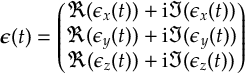
|
(4.1) |
each line consists of 8 elements: t (in fs), ℜ(ϵx(t)), ℑ(ϵx(t)), ℜ(ϵy(t)), ℑ(ϵy(t)), ℜ(ϵz(t)), ℑ(ϵz(t)), (all in atomic units), and finally the instantaneous central frequency (also atomic units).
The time step in the laser file must exactly match the time step used for the electronic propagation, which is the time step used for the nuclear propagation (keyword stepsize) divided by the number of substeps (keyword nsubsteps). The first line of the laser file must correspond to t=0 fs.
Example:
0.00E+00 -0.68E-03  0.00E+00  0.00E+00  0.00E+00  0.00E+00  0.00E+00  0.31E+00
0.10E-02 -0.77E-02  0.00E+00  0.00E+00  0.00E+00  0.00E+00  0.00E+00  0.33E+00
0.20E-02 -0.13E-01  0.00E+00  0.00E+00  0.00E+00  0.00E+00  0.00E+00  0.35E+00
     ...       ...       ...       ...       ...       ...       ...       ...
4.6 Atom mask file
The atom mask file contains for each atom a line with a Boolean entry (“T” or “F”), which indicates whether the atom should be considered in the relevant procedures.
Specifically, the atom masking settings affect the options ekincorrect parallel_vel, reflect_frustrated parallel_vel, and decoherence_scheme edc.
In all cases, “T” indicates that the atom should be considered (as if atommask was not given), whereas “F” indicates that the atom should be ignored for these procedures.
Example:
 T
 T
 F
 F
...
4.7 RATTLE file
The RATTLE file contains a list of all the atom pairs whose interatomic distance should be fixed by the RATTLE algorithm.
In the file, each line should contain two integer numbers that indicate the atom indices of one atom pair.
Atom indices start at 1.
Optionally, some lines can also have a third entry, which is a float with the desired interatomic distance in Bohr units.
If the third entry is not give, then the distance is fixed to the value that is found in the initial geometry file.
Example:
1 3
2 4  2.05
2 5
4.8 Frozen atoms file
The frozen atoms file contains one line per atom, which should be either T (atom is propagated) or F (atom is frozen).
This format is exactly the same as in the atommaskfile (Section 4.6).
The default file name is frozen, which is used with freeze file.
4.9 Thermostat settings file
The thermostat settings file can be used to define the number of thermostat regions, their temperatures, their thermostat parameters, and the assignment of all atoms to the regions.
The file format is
<n_regions>
<n_regions lines with temperatures>
<n_regions lines with all parameters for the thermostat>
<n_atom lines with one region index>
For example, with two regions, the Langevin thermostat, and six atoms, the thermostat file could look like:
2   ! two regions
300.0   ! temperature in K for region 1
500.0   ! temperature in K for region 2
0.01   ! friction coefficient in fs^-1 for region 1
0.05   ! friction coefficient in fs^-1 for region 2
1   ! atom 1 assigned to region 1
1   ! atom 2 assigned to region 1
1
2   ! atom 4 assigned to region 2
2
2
Trailing comments beyond the expected amount of entries per line are ignored.
The default file name is thermostat_settings, which is used with thermostatregions file.
Chapter 5 Output files
This chapter documents the content of the output files of SHARC.
Those output files are output.log, output.lis, output.dat and output.xyz.
For users using NetCDF output via PySHARC, additional output files are output.dat.nc and output_NUC.dat.nc.
5.1 Log file: output.log
The log file output.log contains general information about all steps of the SHARC simulation, e.g., about the parsing of the input files, results of quantum chemistry calls, internal matrices and vectors, etc. The content of the log file can be controlled with the keyword printlevel in the SHARC main input file.
In the following, all printlevels are explained.
Printlevel 0
At printlevel 0, only the execution infos (date, host and working directory at execution start) and build infos (compiler, compile date, building host and working directory) are given.
Printlevel 1
At printlevel 1, also the content of the input file (cleaned of comments and blank lines) is echoed in the log file. Also, the start of each time step is given.
Printlevel 2
At printlevel 2, the log file also contains information about the parsing of the input files (echoing all enabled options, initial geometry, velocity and coefficients, etc.) and about the initialization of the coefficients after the first quantum chemistry calculation. This printlevel is recommended for production calculations, since it is the highest printlevel where no output per time step is written to the log file.
Printlevel 3
This and higher printlevels add output per time step to the log file. At printlevel 3, the log file contains at each time step the data from the velocity-Verlet algorithm (old and new acceleration, velocity and geometry), the old and new coefficients, the surface hopping probabilities and random number, the occupancies before and after decoherence correction as well as the kinetic, potential and total energies.
Printlevel 4
At printlevel 4, additionally the log file contains information on the quantum chemistry calls (file names, which quantities were read, gradient and nonadiabatic coupling vector selection) and the propagator matrix.
Printlevel 5
At printlevel 5, additionally the log file contains the results of each quantum chemistry calls (all matrices and vectors), all matrices involved in the propagation as well as the matrices involved in the gradient transformation. This is the highest printlevel currently implemented.
5.2 Listing file: output.lis
The listing file output.lis is a tabular summary of the progress of the dynamics simulation. At the end of each time step (including the initial time step), one line with 11 elements is printed. These are, from left to right:
- current step (counting starts at zero for the initial step),
- current simulation time (fs),
- current state in the diagonal representation,
- approximate corresponding MCH state (see subsection 8.23.1),
- kinetic energy (eV),
- potential energy (eV),
- total energy (eV),
- total angular momentum [ħ],
- current gradient norm (in eV/Å),
- total sum of populations (called Density in the file),
- current expectation values of the state dipole moment (Debye),
- current expectation values of total spin,
- wall clock time needed for the time step.
The listing file also contains one extra line for each surface hopping or pointer state switching event. For accepted hops, the old and new states (in diagonal representation) and the random number are given. Frustrated hops and resonant hops are also mentioned. Note that the extra line for surface hopping occurs before the regular line for the time step.
The listing file can be plotted with standard tools like GNUPLOT and can be read with data_collector.py.
Energies
The kinetic energy is calculated at the end of each time step (i.e., after surface hopping events and the corresponding adjustments). The potential energy is the energy of the currently active diagonal state. The total energy is the sum of those two.
Expectation values
The gradient norms given in the listing file is calculated as follows:
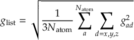
|
(5.1) |
which is then transformed to eV/Å.
The expectation values of the dipole moment for the active state β is calculated from:
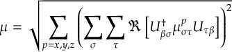
|
(5.2) |
The expectation value of the total spin of the active state β is calculated as follows:
|
(5.3) |
where Sα is the total spin of the MCH state with index α.
5.3 Data file: output.dat
The data file output.dat contains all relevant data from the simulation for all time steps, in ASCII format. Accordingly, this file can become quite large for long trajectories, for many atoms, or if many states are included, but for most file systems it is easier to deal with a single large file than with many small files.
Usually, after the simulation is finished the data file is processed by data_extractor.x to obtain a number of tabular files which can be plotted or post-processed (e.g., with data_collector.py).
For this, see Sections 7.22 for the data extractor, 7.27 for plotting, and 7.36 for post-processing.
Note that if you use NetCDF output, then output.dat will only contain the header information and header arrays.
See Section 5.4 for more details.
5.3.1 Specification of the data file
The data file format was changed between SHARC1 and SHARC2. The new format uses a different header, which is keyword-based (like the input file) and starts with SHARC_version X.Y. The general structure of the time step data is the same as in the first release version.
The data file contains a short header followed by the data per time step. All quantities are commented in the data file.
The header is keyword-based and contains at least the following entries:
- method (surface hopping or CSDM),
- integrator,
- maximum multiplicity,
- number of states per multiplicity,
- number of atoms,
- time step,
- maximum number of time steps,
- number of substeps,
- reference energy,
- write_overlap,
- write_grad,
- write_nacdr,
- write_property1d,
- write_property2d,
- number of 1D properties,
- number of 2D properties,
- information whether a laser field is included.
At the end of the header, the data file contains a header array section. Currently, this includes:
- atomic numbers,
- elements,
- masses,
- full laser field for all substeps (only if flag is set).
The entry for each time step contains:
- step index and current time for adaptive integrators,
- Hamiltonian in MCH representation,
- transformation matrix U,
- MCH dipole moment matrices (x, y, z),
- overlap matrix in MCH representation (only if flag is set),
- coefficients in the diagonal representation,
- hopping probablities in the diagonal representation
- kinetic energy,
- currently active state in diagonal representation and approximate state in MCH representation,
- random number for surface hopping,
- wall clock time (in seconds)
- geometry (Bohrs),
- velocities (atomic units),
- 2D property matrices (only if flag is set),
- 1D property vectors (only if flag is set),
- gradient vectors (only if flag is set),
- nonadiabatic coupling vectors (only if flag is set).
5.4 Data file in NetCDF format: : output.dat.nc
If output_format is set to netcdf, then only the header and header arrays will be written to the output.dat file, but no information per time step.
The latter is instead written in (binary) NetCDF format to output.dat.nc.
This option is intended to provide faster output for fast simulations with pysharc.
However, it is also an option that leads to less disk memory consumption, and can be used with sharc.x.
To this end, output_format=netcdf also deactivates writing of the output.xyz file.
Also, when NetCDF files are written, no restart files are produced, except on the last time step or in case of errors.
NetCDF output files can be extracted with data_extractor_NetCDF.x (see Section 7.23).
This program can also regenerate the output.xyz for further analysis.
Currently, there are a few limitations in this approach.
Most importantly, the NetCDF files do not store the property vectors and property matrices that can be stored in the output.dat files.
Hence, computations with the ionization or theodore keywords should not use the NetCDF format.
Additionally, gradients and nonadiabatic coupling vectors are not written to NetCDF output files.
The program data_converter.x (see Section 7.24) can be used to convert an output.dat file into a NetCDF file.
This can be useful when archiving an ensemble of trajectories, as the NetCDF files are much smaller than the ASCII files.
Note that after conversion, the output.xyz files can be deleted, as they can be regenerated from the NetCDF file.
Conversely, sometimes it is useful to inspect the data manually, which is difficult in NetCDF format.
In this case, one can use data_converter_to_ASCII.x (see Section 7.25), which will produce a file called output.dat.cp (to not overwrite the original output.dat with the header).
5.5 Separate nuclear data file in NetCDF format: output_NUC.dat.nc
With the option output_format netcdf_separate_nuclei, SHARC will split the output data into two NetCDF files.
The files output.dat and output.dat.nc are written as if the system contains only one atom.
Additionally, the file output_NUC.dat.nc is written with only the coordinates and velocities.
Note that output_NUC.dat.nc is not compatible with data_extractor_NetCDF.x or data_converter_to_ASCII.x.
However, it can be read by sharctraj_to_xyz.py (Section 7.8), data_extractor_NUC_xyz.py (Section 7.26), and align_and_reorder_trjaj.py (Section 7.38).
The first of these scripts can be used to extract one time step from the file and write it in xyz, initconds, or geom/veloc formats; this is useful to setup trajectories starting from time steps of a previous trajectory.
The second script extracts the entire output_NUC.dat.nc into XYZ format for visualization and analysis purposes (e.g., with geo.py or geo_NM.py.
The third script can align coordinates in output_NUC.dat.nc files, reorder a trajectory swarm to get NetCDF coordinate files for each time step, and convert the files to a NetCDF format that follows Amber conventions (thus, can be opened by, e.g., VMD or cpptraj).
5.6 XYZ file: output.xyz
The file output.xyz contains the geometries of all time steps in standard xyz file format. It can be used with visualization programs like MOLDEN, GABEDIT or MOLEKEL to create movies of the molecular motion, or with geo.py (see 7.28) to calculate internal coordinates for each time step.
Using geo_NM.py and a normal mode file (V0.txt, see Section 6.4.4 for details), normal mode coordinates can be computed.
Furthermore, trajana_essdyn.py (see 7.35) reads this file.
The comments of the geometries (given in the second line of each geometry block) contain information about the simulation time and the active state (first in diagonal basis, then in MCH basis).
If output_format=netcdf, the output.xyz file will be empty.
Use data_extractor_NetCDF.x (Section 7.23) with the -xyz flag to obtain the output.xyz file.
Conversely, if output_format=netcdf_separate_nuclei is used, the output.xyz file can be generated from output_NUC.dat.nc via the script data_extractor_NUC_xyz.py (Section 7.26).
Chapter 6 Interfaces
This chapter describes the interface between SHARC and any provider of electronic structure information, like potential energy surface models or quantum chemistry programs.
The interface infrastructure of SHARC was completely overhauled in SHARC4, compared to previous versions.
In SHARC3 and previous versions, SHARC interfaces were in principle any script that reads a communication file (QM.in) coming from sharc.x and returning the requested information in a second communication file (QM.out).
On the contrary, in SHARC4 each interface is a Python module implementing a class.
Each interface has a main function that implements the communication via QM.in and QM.out, but additionally each interface also has several methods to instantiate, initialize, execute, and setup a calculation from within Python.
In this way, one can run PySHARC trajectories using driver.py that avoid file I/O for much higher performance.
This dual capability is shown in Figure 6.1.
Additionally, SHARC4 interfaces can call other SHARC4 interfaces, which makes it possible to produce complex workflows in a flexible manner (e.g., QM/MM, numerical gradients, etc).
Note that this interface nesting also applies to setting up of trajectories, where SHARC4 interfaces communicate with the setup scripts by providing the available features and routines to take care of all interface-specific files.
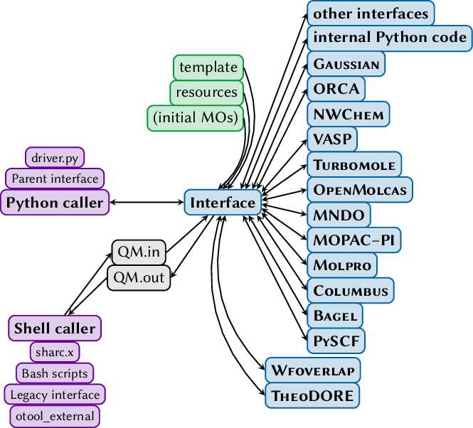
Section 6.0.1 gives a short overview of the existing interfaces.
The subsequent sections document the capabilities of all interfaces.
In Section 6.34, a short specification of the interface is given (for users who want to develop their own interface).
Finally, Section 6.35 provides the documentation for the wfoverlap.x auxiliary program.
6.0.1 Overview over Interfaces
The SHARC4 interfaces are derived from three different base classes: fast interfaces, ab initio interfaces, and hybrid interfaces.
However, this classification is more relevant for interface developers, whereas for users a slightly finer granularity is more useful.
In this way, we can distinguish six different interface kinds of interfaces:
- Stub interfaces are very simply interfaces that do not do file I/O or call an external program, but instead simply return trivial information, like zeros, unit matrices, or constant values. These are mostly intended for testing.
- Fast interfaces implement fast potential energy methods that are evaluated within Python, without file I/O or expensive ab initio computations. Examples include analytical, machine-learning, or molecular mechanics models. These interfaces can run in the so-called persisent mode, where they do not even write files for restart (except on the last time step).
- Ab initio interfaces allow SHARC to communicate with external quantum chemistry programs. These interfaces perform file I/O and use the save directory to store information between time steps (e.g., for orbital restart, wave function overlaps). These interfaces have been reimplemented to follow SHARC4 standards.
- Legacy ab initio interfaces are interfaces that have been directly taken from SHARC3 without extensive reimplementations for SHARC4. They have all capabilities they had in SHARC3. In order to use them in SHARC4, they can be called via SHARC_LEGACY.py, which is a SHARC4-compliant interface that acts as a front-end to the legacy interfaces.
- Single-child hybrid interfaces are interfaces that use a single child interface to do part or most of the work. These allows users to manipulate the electronic structure data on the way between the actual providing interface and the caller. Examples are storing electronic structure data in a data base, adding harmonic restrains, or performing numerical differentiation.
- Multi-child hybrid interfaces are interfaces that use a kindergarden of several child interfaces, e.g., to compute the electronic structure results for only a part of the system. They implement, e.g., QM/MM, excitonic multi-fragment models, or adaptive sampling procedures.
Table 6.1 gives an overview over all interfaces available in SHARC4.
The different features in the table are explained here:
- Energies (H): This is the most basic request and is available from every interface. It is omitted in Table 6.1.
- Spin-orbit couplings (SOC): Adds spin-orbit coupling matrix elements between all electronic states to the electronic Hamiltonian. The relevant spin functions are typically in the spherical representation (i.e., complex-valued and with well-defined MS values) but can also be in another basis (e.g., real-valued spin functions).
- Dipole moments (DM): This requests the entire matrix of electric dipole moments and transition dipole moments between all electronic states. Typically, SHARC4 interfaces will return those in the length representation. For some interfaces, some dipole moments cannot be returned and will thus be zero (e.g., excited-to-excited transition dipole moments for TD-DFT).
- Gradients (GRAD): This requests the entire list of gradients of all electronic states, although the request can also be posed to compute only a subset of all gradients.
- Nonadiabatic coupling vectors (NACDR): This requests the entire matrix of nonadiabatic coupling vectors 〈Ψα|∇→R|Ψβ〉 for all electronic states, although also a subset can be requested.
- Wave function overlaps (OVERLAP): This requests the matrix containing 〈Ψα(t)|Ψβ(t+∆t)〉, computed between the current step and the most recent previous one (using information in the save directory, unless the interface is persistent). Interfaces that can compute overlaps can also serve PHASES requests.
- Dyson norms (ION): This requests the matrix containing the Dyson norms between all electronic states. This is handled by SHARC as a property matrix, which does not affect the dynamics.
- Electronic wave function descriptors (TheoDORE): This requests various descriptors for electronic wave functions (charge transfer, multiconfigurational character, localization, etc), which are treated as sets of property vectors that do not affect the dynamics.
- Electrostatic embedding via point charges (point charges): This is not request, but a feature that some SHARC4 interfaces have. They can receive a set of point charges and perform electrostatic embedding. If gradients or nonadiabatic coupling vectors are requested, also returns those on the point charges.
- Atomic point-multipole representation of electronic densities (multipolar_fit): This requests for each electronic state and each pair of electronic states a set of monopoles+dipoles+quadrupoles per atom that represents the electrostatics of the corresponding state or transition density.
- Molecular wave function information and density matrices (mol/densities): This requests that the atomic orbital basis set and all possible electronic density matrices in the atomic orbital basis are returned.
| Interface | Method | Mult | ||||||||||||
| – Stub interfaces – | ||||||||||||||
| DO_NOTHING | zeros | any | (√) | (√) | (√) | (√) | (√) | (√) | (√) | (√) | (√) | – | 6.1 | pageref |
| QMOUT | constant | any | √ | √ | (√) | (√) | (√) | – | – | – | √ | – | 6.2 | pageref |
| – Fast interfaces – | ||||||||||||||
| ANALYTICAL | sympy | any | √ | √ | √ | √ | √ | – | – | – | – | – | 6.3 | pageref |
| LVC | LVC/QVC models | any | √ | √ | √ | √ | √ | – | – | √ | √ | – | 6.4 | pageref |
| SPAINN | PaiNN models | singlet | – | √ | √ | √ | – | – | – | – | – | – | 6.5 | pageref |
| SCHNARC | SchnArc models | any | √ | √ | √ | √ | – | – | – | √ | – | – | 6.6 | pageref |
| OPENMM | MM force fields | 1 state | – | √ | √ | – | (√) | – | – | – | √ | – | 6.7 | pageref |
| NAI | NaI 2-state model | 2 states | – | √ | √ | – | √ | – | – | – | – | – | 6.8 | pageref |
| – Ab initio interfaces – | ||||||||||||||
| GAUSSIAN | TD-DFT | any | – | √b | √ | – | √ | √ | √ | √ | √ | √ | 6.9 | pageref |
| ORCA | TD-DFT | any | √c | √b | √ | – | √ | √ | √ | √ | √ | √ | 6.10 | pageref |
| BASICORCA | TD-DFT | singlet | – | √b | √ | – | – | – | – | – | – | – | 6.11 | pageref |
| NWCHEM | TD-DFT | any | – | √b | √ | – | √ | – | – | – | – | – | 6.12 | pageref |
| VASP | KS-TD-DFT | singlet | – | (√) | √f | – | √ | – | – | – | – | – | 6.13 | pageref |
| TURBOMOLE | ADC(2), CC2 | any | √c | √ | √ | – | √ | √ | √ | √ | – | – | 6.14 | pageref |
| MOLCAS | RASSCF, CASPT2 | any | √ | √ | √ | √ | √ | √ | √ | √ | √ | √ | 6.15 | pageref |
| MNDO | OMx/MRCI | singlet | – | √ | √ | √ | √ | – | – | √ | – | – | 6.16 | pageref |
| MOPACPI | AM1/FOMO-CI | singlet | – | √ | √ | √ | √ | – | – | –d | – | – | 6.17 | pageref |
| TEQUILA | Quantum computing | singlet | – | √ | √g | √g | √ | – | – | – | – | – | 6.18 | pageref |
| LEGACY | SHARC legacy interface | any | √ | √ | √ | √ | √ | √ | √ | – | – | – | 6.19 | pageref |
| – Legacy ab initio interfaces – | ||||||||||||||
| AMS_ADF | TD-DFT | any | √ | √b | √ | – | √ | √ | √ | – | – | – | 6.20 | pageref |
| COLUMBUS | CASSCF, MRCISD | any | √e | √ | √ | √ | √ | √ | – | – | – | – | 6.21 | pageref |
| BAGEL | CASSCF, (X)MS-CASPT2 | singlet | – | √ | √ | √ | √ | – | – | – | – | – | 6.22 | pageref |
| MOLPRO | CASSCF | any | √ | √ | √ | √ | √ | √ | – | – | – | – | 6.23 | pageref |
| PYSCF | CASSCF, CMS-PDFT | singlet | – | √ | √ | √ | – | – | – | – | – | – | 6.24 | pageref |
| – Single-child hybrid interfaces – | ||||||||||||||
| ASE | save data | Depends on child interface. | 6.25 | pageref | ||||||||||
| UMBRELLA | add restraints | Depends on child interface. | 6.26 | pageref | ||||||||||
| DROPLET | add droplet/tether | Depends on child interface. | 6.27 | pageref | ||||||||||
| CPA | use ground-state gradient | Depends on child interface. | 6.28 | pageref | ||||||||||
| NUMDIFF | finite differences | Depends on child interface. | 6.29 | pageref | ||||||||||
| – Multi-child hybrid interfaces – | ||||||||||||||
| QMMM | el.-stat. embedding | Depends on child interfaces. | 6.30 | pageref | ||||||||||
| ECI | excitonic HF/CI | Depends on child interfaces. | 6.31 | pageref | ||||||||||
| ADAPTIVE | quorum-based | Depends on child interfaces. | 6.32 | pageref | ||||||||||
| Interface | Template file | Resource file | Initial MOs | |
| – Stub interfaces – | ||||
| DO_NOTHING | N/A | |||
| QMOUT | QMOUT.template | N/A | ||
| – Fast interfaces – | ||||
| ANALYTICAL | ANALYTICAL.template | ANALYTICAL.resources | N/A | |
| LVC | LVC.template | LVC.resources | N/A | |
| SPAINN | SPAINN.template | SPAINN.resources | N/A | |
| OPENMM | OPENMM.template | OPENMM.resources | N/A | |
| NAI | N/A | NAI.resources | N/A | |
| – Ab initio interfaces – | ||||
| GAUSSIAN | GAUSSIAN.template | GAUSSIAN.resources | GAUSSIAN.chk.<job>.init | |
| ORCA | ORCA.template | ORCA.resources | ORCA.gbw.<job>.init | |
| BASICORCA | BASICORCA.template | BASICORCA.resources | N/A | |
| NWCHEM | NWCHEM.template | NWCHEM.resources | N/A | |
| VASP | VASP.template | VASP.resources | N/A | |
| TURBOMOLE | TURBOMOLE.template | TURBOMOLE.resources | mos.init | |
| MOLCAS | MOLCAS.template | MOLCAS.resources | MOLCAS.<mult>.RasOrb.init | |
| MOLCAS.<mult>.JobIph.init | ||||
| MNDO | MNDO.template | MNDO.resources | N/A | |
| MOPACPI | MOPAC_PI.template | MOPAC_PI.resources | N/A | |
| TEQUILA | TEQUILA.template | TEQUILA.resources | angles_json.<state>.init | |
| LEGACY | LEGACY.template | LEGACY.resources | N/A | |
| – Legacy ab initio interfaces – | ||||
| AMS_ADF | AMS_ADF.template | AMS_ADF.resources | AMS_ADF.t21.<job>.init | |
| COLUMBUS | a directory | COLUMBUS.resources | mocoef_mc.init.<job> | |
| COLUMBUS | molcas.RasOrb.init.<job> | |||
| BAGEL | BAGEL.template | BAGEL.resources | archive.<mult>.init | |
| MOLPRO | MOLPRO.template | MOLPRO.resources | wf.<job>.init | |
| PYSCF | PYSCF.template | PYSCF.resources | pyscf.init.chk | |
| – Single-child hybrid interfaces – | ||||
| ASE_DB | ASE_DB.template | N/A | ||
| UMBRELLA | UMBRELLA.template | N/A | ||
| DROPLET | DROPLET.template | N/A | ||
| CPA | CPA.template | N/A | ||
| NUMDIFF | NUMDIFF.template | NUMDIFF.resources | N/A | |
| – Multi-child hybrid interfaces – | ||||
| QMMM | QMMM.template | QMMM.resources | N/A | |
| ECI | ECI.template | ECI.resources | N/A | |
| ADAPTIVE | ADAPTIVE.template | ADAPTIVE.resources | N/A | |
| Keyword | Description |
| scratchdir | Is a path to the temporary directory. Relative and absolute paths, environment variables and can be used. If it does not exist, the interface will create it. In any case, the interface will delete this directory after the calculation. |
| savedir | Is a path to another temporary directory. Relative and absolute paths, environment variables and can be used. The interface will store files needed for restart there. Is superseded by the savedir requested by the caller, so this keyword is usually optional in the resource file. |
| retain | Followed by an integer giving the number of old time steps to retain in the step file. Is superseded by the retain setting from the caller, so this keyword is usually optional in the resource file. |
| memory | The memory usable by the interface. Behaviour is interface-specific. |
| ncpu | The number of CPUs used by the interface. Is overridden by environment variables from queuing engines (e.g., $NSLOTS or $SLURM_NTASKS_PER_NODE). Parallel behaviour is interface-specific. |
| min_cpu | Minimum number of CPUs per job. Parallel behaviour is interface-specific. |
| ngpu | The number of GPUs used by the interface. Parallel behaviour is interface-specific. |
| schedule_scaling | Gives the expected parallelizable fraction of the parallezable calculations (Amdahl’s law). With a value close to zero, the interface will try to run all jobs at the same time. With values close to one, jobs will be run sequentially with the maximum number of cores. Exact behaviour is interface-specific. |
| delay | Followed by a float giving the delay in seconds between starting parallel jobs to avoid excessive disk I/O (usually not necessary). |
| always_orb_init | Do not use the orbital guesses from previous calculations/time steps, but always use the provided initial orbitals. |
| always_guess | Always use the orbital guess from the quantum chemistry program. |
| Keyword | Description |
| wfoverlap | Path to the WFOVERLAP code. Needed for overlap and Dyson norm calculations in some interfaces. |
| wfthres | (float) Gives the amount of wave function norm which will be kept in the truncation of the determinant files. Default is interface-specific. |
| numfrozcore | Number of frozen core orbitals for overlap and Dyson norm calculations. A value of -1 enables automatic frozen core. |
| wfnumocc | Number of ignored occupied orbitals in Dyson calculations. |
| nooverlap | Do not save determinant files for overlap computations. |
| theodir | Path to the THEODORE installation. Relative and absolute paths, environment variables and can be used. The interface will set $PYTHONPATH automatically. |
| theodore_prop | Followed by a list with the descriptors which THEODORE should compute. Note that descriptors will only be computed for restricted singlets (and triplets). Instead of a simple list, a Python literal can also be used, as in the THEODORE input files. |
| theodore_fragment | Followed by a list of atom numbers which should constitute a fragment in THEODORE. For multiple fragments, the keyword can be used multiple times. Instead, the keyword can be followed by a Python literal, as in the THEODORE input files. |
| Keyword | Description |
| resp_target | Defines the target for the RESP restraint. Default is ‘zero’, but ‘mulliken’ and ‘lowdin’ can also be used. |
| resp_layers | Number of layers, default 4. |
| resp_first_layer | Factor for the radius of the innermost fitting layer. The other factors are computed as first + 0.4 n−0.5*i for i=0 to n−1. The actual radius of each fitting layer is the product of the factors times the VdW radius of the respective atom. Default is 1.4. Together with the default 4 layers, the layer factors are 1.4, 1.6, 1.8, 2.0 (as, e.g., in Gaussian). |
| resp_density | Fitting point density in points per Å2. Default is 10. |
| resp_fit_order | Integer, 0, 1, or 2 for monopoles-only, monopoles+dipoles, or up to quadrupoles. Default 2. |
| resp_grid | String defining the spherical quadrature used. Possible are ‘lebedev’, ‘random’, ‘golden_spiral’, ‘gamess’, and ‘marcus_deserno’. Default is ‘lebedev’, which is the one with the highest inherent symmetry. |
| resp_betas | Parameters that define the strength of the restraint for the different fitting orders. Defaults are 0.0005, 0.0015, 0.003 for monopoles, dipoles, quadrupoles. See [36]. |
| resp_mk_radii | Use original Merz-Kollman radii for HCNOSP [114]. Default is to use values from Ref. [115] for all atoms. |
| resp_vdw_radii | Provide a list of VdW radii for all atoms, in Python syntax. Has precedence over resp_vdw_radii_symbol. |
| resp_vdw_radii_symbol | Provide a dictionary of VdW radii for all elements, in Python syntax. |
| resp_block_size | Number of blocks fitted simultaneously. Affects memory consumption. Use resp_memory_estimator.py (Section 7.17) to estimate a reasonable block size. |
| resp_nuke_ram | Use the old, memory-heavy fitting routine. Default is False. |
6.0.4 Interface development guide
Users who want to develop their own interfaces for SHARC should inspect the SHARC interface developers guide, a separate PDF available from the SHARC homepage.
It provides a detailed description of what considerations need to be taken when developing an interface.
If developing an ab initio or hybrid interface, developers should also consider basing their work on the provided skeleton code files.
- $SHARC/../examples/SHARC_ABINITIO/SHARC_ABINITIOTEMPLATE.py: skeleton code for a standard ab initio interface, using the standard job scheduling from the ab initio base class.
- $SHARC/../examples/SHARC_HYBRID/SHARC_HYBRIDTEMPLATE.py: skeleton code for a regular single-child hybrid interface.
Note that interface development might involve some non-obvious pitfalls, especially for non-trivial methods.
Interface developers are invited to contact the SHARC developers for collaboration.
6.1 Do-Nothing Interface
Stub interface that returns all zeros.
The SHARC-Do-Nothing interface is a stub interface that returns zeros for all requested quantities (but unit overlaps and unity phases).
In that sense, it supports every request, except for molecule/density matrices.
It is intended as a developers tool and cannot be used to carry out any actual investigations.
The interface does not have any template or resource options and in fact does not even read either file.
During setup, this interface asks a random question and writes the user’s reply to a file in the relevant directory.
This file does not have any effect.
6.2 QMout Interface
Stub interface that returns constant energies and potential-like couplings, and zeros for other requests, for frozen-nuclei dynamics.
The SHARC-QMout interface is a stub interface intended for running dynamics with frozen nuclei, i.e., purely electronic dynamics.
As such, it returns constant energies, spin-orbit couplings, dipole moments, and possibly multipolar density expansions, but otherwise returns zeros (but unit overlaps and unity phases).
Its name stems from the fact that it reads the constant energies, couplings, and other quantities from a QM.out file, as it is produced by all other interfaces.
Note that it ignores all content of this file except for energies, spin-orbit couplings, dipole moments, and multipolar density expansions.
When it is looking for the file, the assumed file name is QMout.template.
The interface has no other options besides the contents of the QMout.template file.
During setup, the interface asks first for the path to a template file.
If this path leads to a QM.out file, it is used as is for all trajectories that are set up.
If this path is a directory containing ICOND folders, then the QM.out file for TRAJ_XXXXX is automatically taken from ICOND_XXXXX.
The interface then asks whether the QM.out files should be copied or linked.
6.3 Analytical PESs Interface
Fast interface for self-coded potential energy surfaces using SymPy.
This interface allows to run dynamics simulations on PESs expressed with analytical functions.
The system Hamiltonian is defined in a diabatic representation, and the interface automatically diagonalizes this Hamiltonian to produce adiabatic states.
If spin-orbit couplings are given, these are treated like in other interfaces (they are not diagonalized away), so that the interface returns data in the MCH representation.
Since SHARC4, this interface requires the Python package sympy.
This package is used to automatically find the derivatives of the Hamiltonian matrix elements, so that the derivatives do not have to be coded by hand, like in older SHARC versions.
The interface needs two additional input files, called ANALYTICAL.template and ANALYTICAL.resources.
The former one contains the definitions of all analytical expressions, the second one contains two optional settings.
In SHARC4, the interface can provide energies, SOCs, gradients, nonadiabatic couplings, overlaps and phases.
The necessary data to compute overlaps with the previous time step are stored in main memory if the interface is in persistent mode, or in the save directory in non-persistent mode. Additionally, (transition)dipole moments can be defined.
6.3.1 Parametrization
The interface has to be provided with analytical expressions for all matrix elements of the following matrices in the diabatic basis:
- Hamiltonian: H
- (Optionally) (Transition) dipole matrices for each polarization direction: Mi
- (Optionally) real and imaginary part of the SOC matrix: Σ
The diabatic Hamiltonian is diagonalized:
|
(6.1) |
Then the following calculations lead to the MCH matrices which are passed to SHARC:

|
(6.2) |
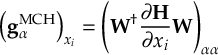
|
(6.3) |
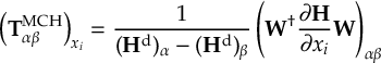
|
(6.4) |
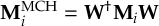
|
(6.5) |
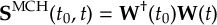
|
(6.6) |
The MCH Hamiltonian is the diagonalized diabatic Hamiltonian plus the SO matrix transformed into the MCH basis.
The gradients in the MCH basis are obtained by transforming the derivative of the diabatic Hamiltonian (computed with sympy) into the MCH basis.
The nonadiabatic coupling vectors are computed likewise.
The dipole matrices are simply transformed into the MCH basis.
The overlap matrix is the overlap of old and new transformation matrix.
6.3.2 Template file: ANALYTICAL.template
The interface-specific input file is called ANALYTICAL.template. It contains the analytical expressions for all matrix elements mentioned above. All analytical expressions in this file are evaluated considering the atomic coordinates read from QM.in or passed by the caller.
The file consists of a file header and the file body.
The file body consists of variable definition blocks and matrix blocks.
A commented template file is located in $SHARC/../examples/SHARC_ANALYTICAL/.
Note that all units are atomic units.
Header
The header looks similar to an xyz file:
2
2
I       xI       0       0
Br      xBr      0       0
Here, the first line gives the number of atoms and the second line the number of states.
Note that this interface ignores whatever system charge is declared by the caller.
On the remaining lines, each Cartesian component of the atomic coordinates is associated to a variable name, which can be used in the analytical expressions.
If a zero (0) is given instead of a variable name, then the corresponding Cartesian coordinate is neglected.
In the above example, the variable name xI is associated with the x coordinate of the first atom given in QM.in.
The y and z coordinates of the first atom are neglected.
All variable names must be valid Python identifiers and must not start with an underscore.
Hence, all strings starting with a letter, followed by an arbitrary number of letters, digits and underscores, are valid.
It is not allowed to use a variable name twice.
Note, that the file header also contains the atom labels, which are just used for cross-checking against the atom labels in QM.in.
The file header must not contain comments, neither at the end of a line nor separate lines. Also, blank lines are not allowed in the header. After the last line of the header (where the variables for the natom-th atom are defined), blank lines and comments can be used freely (except in matrix blocks).
Variable definition blocks
Variable definition blocks can be used to store additional numerical values (beyond the atomic coordinates) in variables, which can then be used in the equations in the matrix blocks. The most obvious use for this is of course to define values which will appear several times in the equations.
A variable definition block looks like:
Variables
A1      0.067
g1      0.996   # Trailing comment
# Blank line with comment only
R1      4.666
End
Each block starts with the keyword “Variables” and is terminated with “End”. In-between, on each line a variable name and the corresponding numerical value (separated by blanks) can be given. Note that the naming conventions given above also apply to variables defined in these blocks.
There can be any number of complete variable definitions blocks in the input file. All blocks are read first, before any matrix expressions are evaluated. Hence, the relative order of the variable blocks and the matrix blocks does not matter. Also, note that variable names must not appear twice, so variables cannot be redefined halfway through the file.
Matrix blocks
The most important information in the input file are of course contained in the expressions in the matrix blocks. In general, a matrix block has the following format:
Matrix_Identifier
V11;
V12;    V22;
V13;    V23;    V33;
...
The first line identifies the type of matrix. Those are valid identifiers:
| Hamiltonian | Defines the Hamiltonian including the diabatic potential couplings. |
| Dipole followed by 1, 2 or 3 | (Transition) dipole moment matrix for Cartesian direction x, y or z, respectively. |
| SOC followed by Re or Im | Real or Imaginary (respectively) part of the spin-orbit coupling matrix Σ. |
Since the interface searches the file for these identifiers starting from the top until it is found, for each matrix only the first block takes effect. Note, that the Hamiltonian must be present. If dipole matrix or SO matrix definitions are missing, they will be assumed zero.
In the lines after the identifier, the expressions for each matrix element are given. Note the lower triangular format (all matrices are assumed symmetric, except the imaginary part of the SO matrix, which is assumed antisymmetric). Matrix elements must be separated by semicolons (so that whitespace can be used inside the expressions), including all end-of-lines (also the last line). There must be at least as many lines as the number of states (additional lines are neglected). If any line or matrix element is missing, the interface will abort.
An exemplary block looks like:
Hamiltonian
A1*( (1.-exp(g1*(R1-xI+xBr)))**2-1.);
0.0006;                                        3e-5*(xI-xBr)**2;
It is important to understand that the expressions are directly evaluated by sympy, hence all expressions must be valid Python/sympy expressions which evaluate to numeric (integer or float) values. Only the variables defined above can be used.
Note that exponentiation in Python is **.
Mathematical functions from sympy, e.g., these elementary functions, are available.
6.3.3 Template file: ANALYTICAL.resources
The resource file of SHARC_ANALYTICAL.py knows only one keyword.
The keyword is diagonalize.
It is true by default, but using diagonalize false, one can turn off diagonalization, so that one can run directly in the diabatic basis.
Note that this will give wrong results if the off-diagonal elements of the Hamiltonian are not constant.
6.3.4 During setup
SHARC_ANALYTICAL.py follows the standard initialization procedure during setup.
The first step is to locate the ANALYTICAL.template input file.
If a file named ANALYTICAL.template exists in the current directory, it is suggested as a default.
Otherwise, the user is prompted to specify the correct path manually.
This is repeated until a valid file is provided.
Once the template file is confirmed, it is automatically scanned for required keywords depending on the type of calculation requested.
If SOC is among the requested properties (e.g., within setup_traj.py), the template file must contain a SOC section.
Likewise, for dipole-related requests (dm or dmdr), the Dipole section must be present.
Once setup is finished, the provided template file is copied or symlinked into the working directory.
Note that the setup routine does not ask for a resource file.
If you require one, you need to create and copy it manually.
6.4 LVC Interface
Fast interface for linear and quadratic vibronic coupling models, also with electrostatic embedding.
The purpose of the LVC interface is to allow performing computationally efficient dynamics using a linear vibronic coupling (LVC) or quadratic vibronic coupling (QVC) model [116].
The relevant equations can be found in Section 8.18.
In SHARC4, the interface can provide energies, SOCs, gradients, nonadiabatic couplings, overlaps, multipolar charges, and deal with point charges.
The necessary data to compute overlaps with the previous time step are stored in main memory if the interface is in persistent mode, or in the save directory in non-persistent mode.
6.4.1 Input files
Two input files are needed:
V0.txt
Contains all information to describe the reference harmonic oscillator V0: the equilibrium geometry, the frequencies ωi, and an orthogonal matrix containing the normal coordinates Kαi.
Geometry
 S     16.    0.00000000    0.00000000   -0.00039079   31.97207180
 O      8.    0.00000000   -2.38362453    1.36159121   15.99491464
 O      8.    0.00000000    2.38362453    1.36159120   15.99491464
Frequencies
 0.0000  0.0000  0.0000  0.0000  0.0000  0.0000  0.00234  0.0053  0.0064
Mass-weighted normal modes
  0.0000  1.0000  0.0000  0.0000  0.0000  0.0000  0.0000  0.0000  0.0000
  0.6564  0.0000  0.0000  0.3108  0.0494  0.2004  0.0000  0.0000 -0.6557
...
Here, the reference geometry is given as element, nuclear charge, Cartesian coordinates (x/y/z, in Bohrs), and mass (in atomic mass units).
The frequencies are given all on one line, in Hartree energy units.
The normal mode transformation matrix is given with one column per normal mode (same order as the frequencies) and with three lines per atom (x/y/z, same order as in the reference geometry).
V0.txt can be created from a MOLDEN file using wigner.py -l.
LVC.template
Contains the state-specific information:
ϵi,
κi(n),
λj(m,n),
γij(m,n),
ηmn,
Λi(m,n),
P(m,n)apb,
as well as (transition) dipole moments (see Section 8.18).
Here, for multiplets most parameters are are shared between the multiplet components, whereas in the SOC and dipole moment matrices the multiplet components are provided explicitly.
V0.txt
4 0 3
epsilon
7
  1   1  0.0000000000
  1   2  0.1640045037
  1   3  0.1781507393
  1   4  0.2500917150
  3   1  0.1341247878
  3   2  0.1645714941
  3   3  0.1700512159
kappa
12
  1   2     7  1.19647e-03
  1   2     8  1.21848e-02
...
lambda
3
  1   1   4     9 -1.83185e-02
  1   2   3     9  7.32022e-03
  3   1   3     9  5.71746e-03
lambda_soc
0
gamma
0
SOC R
  0.000e+00  0.000e+00  0.000e+00  0.000e+00  0.000e+00  0.000e+00 ...
  0.000e+00  0.000e+00  0.000e+00  0.000e+00  0.000e+00 -1.086e-04 ...
...
SOC I
  0.000e+00  0.000e+00  0.000e+00  0.000e+00  0.000e+00  0.000e+00 ...
  0.000e+00  0.000e+00  0.000e+00  1.000e+00  0.000e+00  1.000e-04 ...
...
DMX R
 -7.400e-07 -1.639e-01  0.000e+00  3.000e-06  0.000e+00  0.000e+00  ...
 -1.639e-01  3.930e-06  0.000e+00  2.400e-05  0.000e+00  0.000e+00  ...
...
DMX I
...
DMY R
...
DMY I
...
DMZ R
...
DMZ I
...
Multipolar Density Fit
72
1  1  1   0     -0.081  0.135  0.000 -0.000 -0.114  0.093  0.020 -0.000  0.000 -0.000
1  1  1   1     -0.138 -0.123  0.000 -0.000  0.645 -2.028  1.382  0.000  0.000 -0.000
1  1  1   2      0.109 -0.015 -0.030 -0.000 -0.137  0.161 -0.023  0.089  0.000  0.000
1  1  1   3      0.109 -0.015  0.030  0.000 -0.137  0.161 -0.023 -0.089 -0.000  0.000
1  1  2   0      0.000 -0.000  0.000  0.000  0.000 -0.000 -0.000  0.000 -0.000 -0.297
1  1  2   1     -0.000  0.000 -0.000  0.000 -0.000 -0.000  0.000 -0.000  0.000  2.286
1  1  2   2     -0.000  0.000  0.000  0.119 -0.000  0.000 -0.000 -0.000 -0.038 -0.217
1  1  2   3      0.000  0.000  0.000 -0.119  0.000  0.000 -0.000  0.000  0.038 -0.217
...
Only the three first lines are mandatory, but if no other parameters are given, all states will have the same potentials (the ground state potential).
6.4.2 Resource file
In SHARC4, the interface also got a LVC.resource file.
It only knows four keywords.
The first keyword is diagonalize.
It is true by default, but using diagonalize false, one can turn off diagonalization, so that one can run directly in the diabatic basis.
Note that this will give wrong gradients/NACs if any non-zero λ terms are present.
The second keyword is do_kabsch.
If set to true, the Kabsch algorithm will be used to align the current geometry with the reference geometry.
By default, it is true of point charges are present (i.e., in a QM/MM context).
If set to false, an error will be raised if the initial geometry does not match with the reference geometry.
The third keyword is do_permutation.
If set to true, the interface will read the fourth keyword, equivalent_groups_of_atoms, as a list of list of atom indices (starting at zero).
Each inner list designates a set of equivalent atoms, e.g., the hydrogen atoms of a methyl group.
If set to true, during the first time step, the interface attempts to permute the atoms inside each designated set to minimize the RMSD with the reference structure of that group.
A permutation index will be generated and applied to the input coordinates and (inverted) to the output gradients, NAC vectors, and multipolar fit data.
In this way, if the user has initial conditions from some classical MD trajectories where methyl groups can freely rotate, the interface can resolve such groups and run dynamics without the user manually needing to reassign the methyl groups.
6.4.3 During setup
SHARC_LVC.py follows the standard initialization procedure during setup.
The first step is to locate the LVC.template input file.
If a file named LVC.template exists in the current directory, it is suggested as a default.
Otherwise, the user is prompted to specify the correct path manually.
This process is repeated until a valid file is provided.
Once the template file is confirmed, it is automatically scanned for required sections based on the requested properties.
For spin-orbit coupling (soc), either SOC or lambda_soc must appear in the template.
If dipole moments are requested (dm), the file must contain a DM section.
Requests involving point_charges or multipolar_fit require the presence of the Multipolar Density Fit section.
If any required section is missing, the setup terminates with an error.
After the template check, the user is asked whether an LVC.resources file is available.
If so, the file path must be specified.
If not, the user is prompted whether to enable the Kabsch algorithm, which aligns molecular geometries.
If selected, a simple resource file containing the line do_kabsch true is created automatically in the working directory during preparation.
As in the analytical interface, the setup routine copies or symlinks all required files into the working directory.
6.4.4 Template File Setup: wigner.py, setup_LVCparam.py, create_LVCparam.py, modify_LVC_template.py
Reference potential
V0.txt is created using the wigner.py script, which is also used for initial condition generation. Simply call, e.g.
$SHARC/wigner.py -l <filename.molden>
Note that this best works if all 3N normal modes are present in the file.
If the translations and rotations are missing, the script will add the necessary number of zero-vector modes.
If you experience a failure in wigner.py, please try first to provide a molden file with sufficient numerical precision.
It is also advisable to properly symmetrize the relevant frequency calculation.
Setup for single point calculations
To obtain the LVC parameters, two steps are necessary: (i) running quantum chemistry calculations, and (ii) converting the quantum chemistry output to the LVC parameters.
The first of these steps is carried out with setup_LVCparam.py.
It is an interactive script that works very similarly to the other setup scripts (e.g., setup_init.py, setup_traj.py).
The script will ask for the following:
- Path to the V0.txt file,
- Number of states,
- Charge per multiplicity,
- Which interface to use (in principle, all SHARC-interfaces can be used, but only the ab initio interfaces are useful here),
- Whether spin-orbit couplings should be calculated (only if applicable),
- Whether linear SOC terms should be computed (only if applicable),
- Whether κ parameters should be obtained from analytical gradients or numerical differentiation (depends on availability of analytical gradients),
- Whether to compute intrastate quadratic terms γii(αα) (other γ terms cannot be obtained automatically at this time) and how they are computed,
- Whether to compute γii(αα) only for selected states (only if applicable),
- Whether λ parameters should be obtained from analytical nonadiabatic coupling vectors or numerical differentiation (depends on availability of analytical nonadiabatic coupling vectors),
- Which normal modes to include,
- Which normal modes to consider for quadratic terms γii(αα) (only if applicable),
- Which displacement value to use for numerical differentiation (default 0.05 dimensionless mass-frequency scaled units),
- Whether intruder states should be ignored or not,
- Whether one- or two-sided differentiation should be done,
- Whether multipolar charges should be included for LVC/MM,
- Interface-specific input for the chosen quantum chemistry interface (see in the individual interface’s sections in Chapter 6).
The script will set up a directory (DSPL_RESULTS) with one subdirectory for each single point calculation.
If all terms are computed analytically, then only the DSPL_000_eq subdirectory will be present.
Otherwise, for each chosen normal mode 1-2 subdirectories (for one-sided or two-sided differentiation) will be present (possibly more if γ terms are requested).
Additionally, displacements.log presents the most important settings.
In all cases, displacements.json is also present; this file is crucial to communicate all settings to the read-out script after the single point jobs are finished.
Creating LVC parameter files
After all jobs are successfully finished (QM.out file present in each directory), run create_LVCparam.py inside the DSPL_RESULTS directory.
This is a fully automatic script that reads displacements.json and the QM.out files in the subdirectories.
After everything is successfully read, it creates the LVC.template file.
This file can be used to run SHARC-LVC trajectories.
Modifying LVC parameters
Sometimes, one wants to remove certain normal modes or diabatic states from an LVC model, e.g., to investigate the influence of these modes/states.
This can be done with the command line tool modify_LVC_template.py.
A tooltip is available with the -h option.
Currently, it is only possible to remove the highest diabatic states in each multiplicity.
For example, a template file with 4 singlets and 3 triplets can be reduced to the lowest 2 singlets and 2 triplets.
In contrast, any modes can be removed by providing a selection string.
For example, "712,14,1589" selects modes 7-12, 14, and 15-89, i.e., it removes modes modes 1-6, 13, and any modes after 89.
The script also has the three options -no-transition-multipoles, -no-es2es-transition-multipoles, as well as -no-es2es-transition-multipoles-for-mult that can be used to remove multipolar charges that represent transition densities.
6.4.5 Vibronic spectra from VC models: FCClasses_from_LVC.py
The script FCClasses_from_LVC.py uses a set of LVC parameters to compute vibronic spectra via FCClasses.[49]
After an LVC parametization is complete and the V0.txt and LVC.template files have been generated, run FCClasses_from_LVC.py to generate the FCclasses input file and write the parameters in FCclasses-readable format.
Usage
sharctraj_to_xyz.py is an interactive command-line tool and is executed as follows:
user@host> $SHARC/FCClasses_from_LVC.py
It asks the following questions:
- Path to a V0.txt file
- Path to a LVC.template file
- Index of the initial state (e.g., the ground state)
- Index of the final state (e.g., an excited singlet state)
Input
The input V0.txt and LVC.template files need to follow the normal SHARC LVC conventions.
The script uses the ε, κ, and dipole moment parameters.
Output
The script writes all needed input files for FCClassses: freq1.txt, freq2.txt, grad1.txt, grad2.txt, eldip_fchk, and fcc.inp.
To run FCClasses, run:
user@host> fcclasses3 fcc.inp
6.5 SPaiNN Interface
Fast interface to run machine learning potential energy surface models based on the PaiNN architecture.
The SHARC– SPAINN interface allows to run SHARC simulations with machine learning potentials using SchNetPack 2.0.
Neither spin-orbit couplings or overlaps can be computed, but NACs are available.
The interface needs two additional input files, a template file for the quantum chemistry (file name is SPAINN.template) and a resource file (SPAINN.resources). For more information on how to use SPaiNN visit the SPaiNN documentation.
6.5.1 Template file: SPAINN.template
This file contains the specifications for the machine learning potential prediction. The file only contains a number of keywords, given in table 6.6.
A fully commented template file-with all possible options, a comprehensive descriptions, and some practical hints-is located in $SHARC/../examples/SHARC_SPAINN/SPAINN.template.
We recommend that users start from this template file and modify it appropriately for their calculations.
To install SPaiNN clone the repository from GitHub and install with pip.
    git clone https://github.com/CompPhotoChem/SPaiNN.git
    cd SPaiNN
    pip install .
| Keyword | Description |
| cutoff | Cutoff radius for the cutoff function. Note: This should match with the cutoff radius used for training! |
| nac_key | “nacs” or ßmooth_nacs”. |
| properties | List of properties that will be predicted. E.g. [ënergy”, “forces”, “dipoles”, “nacs”] |
6.5.2 Resource file: SPAINN.resources
The file SPAINN.resources contains only the path to the SPaiNN model.
| Keyword | Description |
| modelpath | Path to the trained SPaiNN model. Note that the model cannot be easily verified by the interface at the start. You will obtain an error if you request more states than are in the model or properties that the model cannot predict. |
6.5.3 During setup
SHARC_SPAINN.py follows the standard initialization procedure during setup.
The setup begins by locating the SPAINN.template input file.
If a file with this name exists in the current directory, the user is asked whether it should be used.
If no such file is present, or the user declines, a valid path must be specified manually.
This process is repeated until a valid file is provided.
Note that the machine learning model that is referenced in the template file will not be validated.
Next, the user is asked whether a SPAINN.resources file is available.
If so, the path to this file must be entered, and the file must exist.
If no such file is available, the user is prompted for the location of a trained SPaiNN model via the modelpath field.
During preparation, the provided template is copied or symlinked into the working directory.
If a resource file was provided during setup, it is also copied or linked.
Otherwise, a new SPAINN.resources file is created automatically containing the modelpath.
6.6 SCHNARC Interface
Fast interface to run machine learning potential energy surface models based on the Schnet and FieldSchnet architectures.
The SHARC– SCHNARC interface allows to run SHARCsimulations with machine learning potentials using SchNetPack 1.0.
While the interface is principally able to deliver NACs and spin-orbit couplings (like previous versions), this functionality in the current version has not been tested.
We therefore recommend to use the time derivative based couplings (coupling ktdc), also because couplings between different states are notoriously hard to train.
Since ML machine learned potentials do provide a wave function, overlaps cannot be computed.
This interface can accept point charges and uses the FieldSchNet approach to perform a form of electrostatic embedding.
The interface needs two additional input files, a template file for the quantum chemistry (file name is SCHNARC.template) and a resource file (SCHNARC.resources).
To install SchNarc you first should clone SchNetPack 1.0 from Github.
You can then clone SchNarc from Github.
The installation guide provided on the website is for an older SHARC version, so we do not recommend following it.
Instead use pip to install the package.
If you want to use electrostatic embedding in order to run QM/MM simulations, you have to install FieldSchNet and use the files from Zenodo substituting the ones from SchNarc.
6.6.1 Template file: SCHNARC.template
This file contains the specifications for the machine learning potential prediction.
A fully commented template file-with all possible options, a comprehensive descriptions, and some practical hints-is located in $SHARC/../examples/SHARC_SCHNARC/SCHNARC.template.
We recommend that users start from this template file and modify it appropriately for their calculations.
6.6.2 Template file: SCHNARC.template
The file SCHNARC.template contains only the keyword modelpath, which is the path to the SchNarc model.
This should ideally be an absolute path.
6.6.3 During setup
SHARC_SCHNARC.py follows the standard initialization procedure during setup.
The setup process begins by identifying the SCHNARC.template file.
If this file is found in the current directory, the user is asked whether it should be used.
If not, or if declined, the user must manually provide a valid path to the template file.
This continues until a valid file is confirmed.
The template file has only a single keyword, which is modelpath, which specifies the path to the a pytorch model using either the SCHNARC or FieldSchNet architecture.
During preparation, the template file is either copied or symlinked into the working directory, depending on the configuration.
6.7 OpenMM Interface
Fast interface for molecular mechanics force fields via the OpenMM package, for one state.
This interface implements molecular mechanics force fields using OpenMM.
Given the nature of force fields, this interface can only provide results for a single state which formally is assumed a singlet.
The interface is written to work with AMBER-style prmtop files.
In SHARC4, the interface can provide energies, dipole moments, gradients, and multipolar charges (although only monopole terms will be nonzero).
6.7.1 Template file
The template file OPENMM.template only knows one keyword, prmtop, which provides the path to the prmtop file that defines the system and force field.
In principle, any prmtop file generated with tleap or other AMBERTOOLS should be compatible with the interface, given that the topology is correct.
Prmtop files for QM/MM calculations can be created with setup_from_prmtop.py, see Section 7.16.
6.7.2 Resource file
The resource fileOPENMM.resources knows two keywords.
The first is ncpu, which defines the number of CPU cores to be used.
The second is cuda_device, which accepts an integer that defines the CUDA device to be used.
If this keyword is given, OpenMM is switched from the CPU platform to the CUDA platform.
6.7.3 During setup
SHARC_OPENMM.py follows the standard setup procedure used by other interfaces.
The user is prompted to specify the path to the OPENMM.template file.
The system will attempt to read the specified file using its internal parser.
If any issue arises (e.g., invalid formatting, missing files, etc.), the parser is reset and the user is asked again.
This process repeats until a valid template is provided.
From the parsed template, the necessary prmtop file is extracted and stored as an extra input file.
Finally, the user is asked whether they have an OPENMM.resources file.
If confirmed, they must provide a valid path to it.
During the preparation phase, all required files (template, prmtop, and optional resources) are either copied or symlinked into the working directory depending on the configuration.
6.8 NaI Interface
Fast interface implementing a 2-state model for the molecule NaI.
This interface implements an analytical 2-state, 2-atom model for the molecule NaI, as given in the literature.[117,[47]
This interface will produce an error if there are not exactly two singlet states or not exactly two atoms, one Na and one I.
The interface computes adiabatic energies, gradients, the transition dipole moment, and wave function overlaps.
6.8.1 Template file
This interface does not read a template file.
All parameters are hard-coded.
6.8.2 Resource file
The resource fileNAI.resources knows two keywords.
The keyword diagonalize (default True) allows choosing between diabatic and adiabatic potentials.
The diabatic mode is a test mode.
The keyword keep_U produces a file U_0-NNN.npy in the save directory, containing all transformation matrices.
This is useful for a posteriori diabatization analyses.
6.8.3 During setup
This interface does not ask for any input during setup.
The two options in the resource file need to be manually added if desired.
6.8.4 Analytical model
For completeness, here is the description of the analytical model for NaI:
The diabatic Hamiltonian is defined as
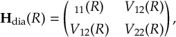
|
(6.7) |
where the adiabatic potential energy surfaces (PESs) are obtained as the eigenvalues of Hdia(R).
R is the Na-I distance.
The analytical forms of the diabatic matrix elements are [117,[47,[46]:
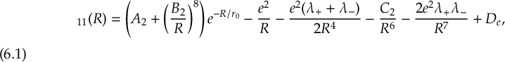 |
(6.8) |
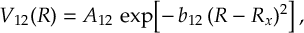 |
(6.9) |
 |
(6.10) |
The diabatic transition dipole moment is defined as a constant off-diagonal element directed along the internuclear axis,
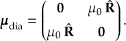 |
(6.11) |
The parameters used in Eqs. (6.8) to (6.11) are as follows.
For the second potential, we use A2 = 2760.0 eV, B2 = 2.398 eV1/8·Å, and C2 = 11.3 eV·Å6, together with λ+ = 0.408 Å3 and λ− = 6.431 Å3.
The equilibrium distance and well depth are given by r0 = 0.3489 Å and De = 2.075 eV, respectively, while the Coulomb prefactor is e2 = 14.3996 eV·Å.
For the first potential, the parameters are A1 = 0.813 eV, b1 = 4.08 Å−1, and R0 = 2.67 Å.
The coupling terms are defined by A12 = 0.055 eV, b12 = 0.6931 Å−2, and Rx = 6.93 Å.
Finally, the dipole parameter is μ0 = 0.1 a.u.
6.9 GAUSSIAN Interface
Ab initio interface for TD-DFT in Gaussian 16.
The SHARC– GAUSSIAN interface allows to run SHARC simulations with GAUSSIAN‘s TD-DFT functionality.
The interface is compatible with restricted and unrestricted ground states (i.e., with all multiplicities), but not with symmetry.
Spin-orbit couplings cannot be computed, but wave function overlaps from the WFOVERLAP code are available (no nonadiabatic couplings).
Dyson norms can also be computed through the WFOVERLAP code.
THEODORE (version 2.0 or higher) can be used to perform automatic wave function analysis.
Furthermore, in SHARC4 the interface can do electrostatic embedding with point charges (gradients on point charges available).
Finally, it can extract and return a PYSCF mol object (containing the atomic orbital basis set) and corresponding one-particle (state/transition) density matrices, as well as multipolar fits of these density matrices.
The interface needs two additional input files, a template file for the quantum chemistry (file name is GAUSSIAN.template) and a resource file (GAUSSIAN.resources).
If files QM/GAUSSIAN.chk.init or QM/GAUSSIAN.chk.<job>.init are present, they are used to provide an initial orbital guess for the SCF calculation of the respective job.
6.9.1 Template file: GAUSSIAN.template
This file contains the specifications for the quantum chemistry calculation. Note that this is not a valid GAUSSIAN input file. The file only contains a number of keywords, given in table 6.8. The actual input for GAUSSIAN will be generated automatically through the interface.
A fully commented template file-with all possible options, a comprehensive descriptions, and some practical hints-is located in $SHARC/../examples/SHARC_GAUSSIAN/GAUSSIAN.template.
We recommend that users start from this template file and modify it appropriately for their calculations.
| Keyword | Description |
| basis | Gives the basis set for all atoms (default def2svp). Note that wave function overlaps are likely wrong with Pople basis sets and other basis sets with shared SP shells (e.g., STO-3G). |
| functional | followed by one string giving the exchange-correlation functional. Default is PBEPBE. |
| dispersion | Activates dispersion correction. Arguments are written verbatim to GAUSSIAN input (in EmpiricalDispersion=()). Default is no dispersion. An example argument would be GD3. |
| scrf | Activates solvation. All arguments (e.g., iefpcm solvent=water) are copied to GAUSSIAN input (in scrf=()). |
| grid | Followed by a string (e.g., grid finegrid) defining which integration grid and accuracy to use. For details, see the example template file. |
| denfit | Activates density fitting, which might speed up the computation. |
| scf | Arguments are written verbatim to GAUSSIAN input (in scf=()). |
| no_tda | This keyword deactivates TDA, which the interface requests by default. |
| td_conv | This sets the TD-DFT convergence threshold to 10−X. Default is 6. |
| unrestricted_triplets | Requests that the triplets are calculated in a separate job from an unrestricted ground state. Default is to compute triplets as linear response of the restricted singlet ground state. |
| noneqsolv | Adds noneqsolv to the td=() block. |
| neglected_gradient | String that is ‘zero’, ‘gs’, or ‘closest’ (default ‘zero’) to control how non-requested gradients are set. |
| state_densities | Uses density=current for all dipole moments and state densities. |
| iop | Arguments are written verbatim to GAUSSIAN input (in iop=()). Expert option. |
| keys | Arguments are written verbatim to GAUSSIAN input as separate keywords. Expert option. |
| basis_external | Pastes the content of the given file after the geometry in the GAUSSIAN input file. Also sets the basis set to gen. Expert option. |
| paste_input_file | Pastes the content of the given file after the external basis block in the GAUSSIAN input file. Expert option. |
6.9.2 Resource file: GAUSSIAN.resources
The file GAUSSIAN.resources contains mainly paths (to the GAUSSIAN executables, to the scratch directory, etc.) and other resources, plus settings for wfoverlap.x and THEODORE. This file must reside in the same directory where the interface is started. It uses a simple “keyword argument” syntax. Comments using # and blank lines are possible, the order of keywords is arbitrary. Lines with unknown keywords are ignored, since the interface just searches the file for certain keywords.
The GAUSSIAN interface employs essentially all keywords from Tables 6.3, 6.4, and 6.5 (except: ngpu), as it uses WFOVERLAP, THEODORE, as well as the RESP module.
Interface-specific keywords are given in Table 6.9.
A fully commented resource file with possible options and descriptions is located in $SHARC/../examples/SHARC_GAUSSIAN/.
| Keyword | Description |
| groot | Is the path to the GAUSSIAN installation directory. This directory should contain the GAUSSIAN executables, e.g., g09/g16, l9999.exe, etc. Relative and absolute paths, environment variables and can be used. The interface will set $GAUSS_EXEDIR to this path. |
| dry_run | If set to true, will not clean the scratchdir, write input files, or run Gaussian calculations. It will perform overlap, TheoDORE, and RESP calculations, and parse output. |
Parallelization
GAUSSIAN usually shows very good parallel scaling for most TD-DFT calculations.
However, it is more efficient to carry out multiple GAUSSIAN calculations (different multiplicities, multiple gradients) in parallel, each one using a smaller number of CPUs.
In the SHARC– GAUSSIAN interface, parallelization is controlled by the keywords ncpu, schedule_scaling, and min_cpu.
The first keyword controls the maximum number of CPUs which the interface is allowed to use for all GAUSSIAN runs simultaneously.
The second keyword is the parallel fraction from Amdahl’s Law, see Section 8.3.
With a value close to zero, the interface will try to run all jobs at the same time. With values close to one, jobs will be run sequentially with the maximum number of cores.
Typical values for schedule_scaling are around 0.90 for both GGA functionals and hybrid functionals, possibly less for very small computations.
The third keyword defines how many cores to use at least for each calculation.
6.9.3 During setup
The GAUSSIAN interface setup begins with the specification of the GAUSSIAN root directory.
The script first attempts to retrieve the path from environment variables ($g16root or $g09root).
If not found, it prompts the user to manually input the path, expanding the path if necessary.
Next, the user is asked to specify a scratch directory for the GAUSSIAN calculations.
Note that the path is not validated by the script, as the calculations may be run on a different machine.
The script will then check for the presence of a valid GAUSSIAN.template file.
If a valid file is detected, the user is prompted to confirm if it should be used.
Otherwise, the user must specify the path to a valid template file.
While specifying the template file, the script also checks if additional files are referenced within the template, such as basis_external or paste_input_file, and adds them to the list of files for setup.
The user is then prompted to provide a restart file (GAUSSIAN chk file) for initial orbitals molecular orbitals.
This is optional.
Finally, the script checks if the user has a GAUSSIAN.resources file.
If the user does not have one, the script will ask for information (number of CPUs, parallel scaling, and memory) in order to generate a new resources file.
The interactive setup of the resource file also allows users to setup the required settings for wave function overlap calculations (path to wfoverlap.x and wave function truncation threshold) and for TheoDORE wave function analysis (path to TheoDORE, property list, and fragment list).
6.9.4 Extracting normal modes: GAUSSIAN_freq.py
This script reads a Gaussian output file from a frequency calculation (requires freq=hpmodes) and generates a Molden file.
These files can be visualized or fed into wigner.py and wigner_state_selected.py.
The idea of this script is to provide a higher numerical precision of the normal mode vectors, compared to the alternative of opening a normal Gaussian output file in Molden and saving it in Molden format.
The usage is:
$SHARC/GAUSSIAN_freq.py GAUSSIAN.log
The script takes the output from the Standard orientation section.
If you want to use the input orientation, use NoSymmetry.
6.10 ORCA Interface
Ab initio interface for TD-DFT in ORCA 5 and 6.
The SHARC– ORCA interface allows to run SHARC simulations with ORCA‘s TD-DFT functionality.
The interface is compatible with restricted and unrestricted ground states (i.e., with all multiplicities), but not with symmetry.
Spin-orbit couplings can be computed and wave function overlaps from the WFOVERLAP code are available (no nonadiabatic couplings).
Dyson norms can also be computed through the WFOVERLAP code.
THEODORE (version 2.0 or higher) can be used to perform automatic wave function analysis.
Furthermore, in SHARC4 the interface can do electrostatic embedding with point charges (gradients on point charges available).
Finally, it can extract and return one-particle (state/transition) density matrices, as well as multipolar fits of these density matrices.
The interface works with ORCA 5 and 6.
The interface needs two additional input files, a template file for the quantum chemistry (file name is ORCA.template) and a resource file (ORCA.resources).
If files QM/ORCA.gbw.init or QM/ORCA.gbw.<job>.init are present, they are used to provide an initial orbital guess for the SCF calculation of the respective job.
6.10.1 Template file: ORCA.template
This file contains the specifications for the quantum chemistry calculation. Note that this is not a valid ORCA input file. The file only contains a number of keywords, given in table 6.10. The actual input for ORCA will be generated automatically through the interface.
A fully commented template file-with all possible options, a comprehensive descriptions, and some practical hints-is located at $SHARC/../examples/SHARC_ORCA/ORCA.template.
We recommend that users start from this template file and modify it appropriately for their calculations.
| Keyword | Description |
| basis | Gives the basis set for all atoms (default 6-31G). |
| auxbasis | Gives the auxiliary basis set (default: Orca chooses). |
| basis_per_element | Overrides the basis set for the specified element (argument 1: element symbol, argument 2: basis set). Can be given multiple times. |
| basis_per_atom | Overrides the basis set for the specified atom (argument 1: atom number starting at 1, argument 2: basis set). Can be given multiple times. |
| ecp_per_element | Overrides the ECP for the specified atom (ECP). Can be given multiple times. |
| functional | followed by one string giving the exchange-correlation functional. Default is PBE. |
| hfexchange | Modifies the amount of HF exchange in the functional (give in fraction of 1). Default is whatever the chosen functional uses. |
| dispersion | Activates dispersion correction. Arguments are written verbatim to ORCA input. Default is no dispersion. |
| no_tda | This keyword deactivates TDA, which the interface requests by default. |
| unrestricted_triplets | Requests that the triplets are calculated in a separate job from an unrestricted ground state. Default is to compute triplets as linear response of the restricted singlet ground state. |
| neglected_gradient | String that is ‘zero’, ‘gs’, or ‘closest’ (default ‘zero’) to control how non-requested gradients are set. |
| ri | Controls the density fitting scheme. Arguments can be, e.g., rijcosx. If not given, RI is decided by ORCA defaults. |
| maxiter | Maximum iterations in ORCA SCF. Default 700. |
| keys | Arguments are written verbatim to ORCA input as separate keywords. Use this to activate CPCM, ZORA, set grid sizes, etc. Expert option. |
| paste_input_file | Path to a file whose content is pasted verbatim into the end of the ORCA input. Expert option. We recommend to use an absolute path here. |
6.10.2 Resource file: ORCA.resources
The file ORCA.resources contains mainly paths (to the ORCA executables, to the scratch directory, etc.) and other resources, plus settings for wfoverlap.x and THEODORE. This file must reside in the same directory where the interface is started. It uses a simple “keyword argument” syntax. Comments using # and blank lines are possible, the order of keywords is arbitrary. Lines with unknown keywords are ignored, since the interface just searches the file for certain keywords.
The ORCA interface employs essentially all keywords from Tables 6.3 (except: ngpu) and 6.4, as it uses WFOVERLAP, THEODORE.
Interface-specific keywords are given in Table 6.11.
A fully commented resource file with possible options and descriptions is located in $SHARC/../examples/SHARC_ORCA/.
| Keyword | Description |
| orcadir | Is the path to the ORCA installation directory. This directory should contain executables like orca, orca_int, or orca_fragovl. Relative and absolute paths, environment variables and can be used. The interface will automatically update the $LD_LIBRARY_PATH. |
| dry_run | If set to true, will not clean the scratchdir, write input files, or run ORCA calculations. It will perform overlap, TheoDORE, and RESP calculations, and parse output. |
Parallelization
ORCA usually shows very good parallel scaling for most TD-DFT calculations.
In the interface, only one ORCA input is written for each multiplicity, as all gradients can be computed in one job.
Hence, schedule_scaling has rarely any effect.
6.10.3 During setup
The ORCA interface setup begins with the specification of the ORCA root directory.
The script prompts the user to manually input the path, expanding the path if necessary.
Next, the user is asked to specify a scratch directory for the ORCA calculations.
Note that the path is not validated by the script, as the calculations may be run on a different machine.
The script will then check for the presence of a valid ORCA.template file.
If a valid file is detected, the user is prompted to confirm if it should be used.
Otherwise, the user must specify the path to a valid template file.
Note that the ORCA interface’s setup routine will not copy extra input files (e.g., used with paste_input_file), so one should use an absolute path in the template file.
The user is then prompted to provide a restart file (ORCA gbw file) for initial orbitals molecular orbitals.
This is optional.
Finally, the script checks if the user has a ORCA.resources file.
If the user does not have one, the script will ask for information (number of CPUs, parallel scaling, and memory) in order to generate a new resources file.
The interactive setup of the resource file also allows users to setup the required settings for wave function overlap calculations (path to wfoverlap.x and wave function truncation threshold) and for TheoDORE wave function analysis (path to TheoDORE, property list, and fragment list).
6.10.4 Extracting normal modes: ORCA_hess_freq.py
This script reads an ORCA Hessian file (e.g., orca.hess) from a frequency calculation and generates a Molden file.
These files can be visualized or fed into wigner.py and wigner_state_selected.py.
The idea of this script is to provide a higher numerical precision of the normal mode vectors, compared to reading them from ORCA’s standard output.
Additionally, .hess files from ORCA are in a consistent format independent of whether symmetry was used or not.
Hence, with ORCA_hess_freq.py, normal modes from frequency calculations with explicit symmetry can be converted to Molden format and used in SHARC.
This is especially beneficial for constructing LVC models (with setup_LVCparam.py and create_LVCparam.py).
The usage is:
$SHARC/ORCA_hess_freq.py ORCA.hess
6.11 BASIC ORCA Interface
Ab initio interface for TD-DFT in ORCA 5 to be used as interface development example.
The SHARC– BASIC ORCA interface allows to run SHARC simulations with ORCA‘s TD-DFT functionality.
As the interface is only intended as a development guideline, it does not have most of the functionality of SHARC_ORCA.py.
SHARC_BASICORCA.py can only provide energies, gradients, and dipole moments.
The interface needs two additional input files, a template file for the quantum chemistry (file name is BASICORCA.template) and a resource file (BASICORCA.resources).
If files QM/BASICORCA.gbw.init or QM/BASICORCA.gbw.<job>.init are present, they are used to provide an initial orbital guess for the SCF calculation of the respective job.
6.11.1 Template file: BASICORCA.template
This file contains the specifications for the quantum chemistry calculation. Note that this is not a valid ORCA input file. The file only contains a number of keywords, given in table 6.12. The actual input for ORCA will be generated automatically through the interface.
A fully commented template file-with all possible options, a comprehensive descriptions, and some practical hints-is located at $SHARC/../examples/SHARC_BASICORCA/BASICORCA.template.
We recommend that users start from this template file and modify it appropriately for their calculations.
| Keyword | Description |
| basis | Gives the basis set for all atoms (default 6-31G). |
| functional | followed by one string giving the exchange-correlation functional. Default is PBE. |
6.11.2 Resource file: BASICORCA.resources
The file BASICORCA.resources contains mainly paths (to the ORCA executables, to the scratch directory, etc.) and other resources. This file must reside in the same directory where the interface is started. It uses a simple “keyword argument” syntax. Comments using # and blank lines are possible, the order of keywords is arbitrary. Lines with unknown keywords are ignored, since the interface just searches the file for certain keywords.
The BASIC ORCA interface employs the keywords from Table 6.13.
A fully commented resource file with possible options and descriptions is located in $SHARC/../examples/SHARC_BASICORCA/.
| Keyword | Description |
| orcadir | Is the path to the BASIC ORCA installation directory. This directory should contain executables like orca, orca_int, or orca_fragovl. Relative and absolute paths, environment variables and can be used. The interface will automatically update the $LD_LIBRARY_PATH. |
6.11.3 During setup
The BASICORCA interface setup begins with the specification of the BASICORCA root directory.
The script prompts the user to manually input the path, expanding the path if necessary.
Next, the user is asked to specify a scratch directory for the ORCA calculations.
Note that the path is not validated by the script, as the calculations may be run on a different machine.
The script will then check for the presence of a valid BASICORCA.template file.
If a valid file is detected, the user is prompted to confirm if it should be used.
Otherwise, the user must specify the path to a valid template file.
Note that the ORCA interface’s setup routine will not copy extra input files (e.g., used with paste_input_file), so one should use an absolute path in the template file.
Finally, the script checks if the user has a BASICORCA.resources file.
If the user does not have one, the script will ask for information in order to generate a new resources file.
6.12 NWCHEM Interface
Ab initio interface for TD-DFT in NWCHEM 7.2.
The SHARC– NWCHEM interface allows to run SHARC simulations with NWCHEM‘s TD-DFT functionality.
The interface is compatible with restricted and unrestricted ground states (i.e., with all multiplicities), but not with symmetry.
Triplets have to be computed as response of a triplet ground state.
Spin-orbit couplings are not available, but wave function overlaps from the WFOVERLAP code are available (no nonadiabatic couplings).
The interface needs two additional input files, a template file for the quantum chemistry (file name is NWCHEM.template) and a resource file (NWCHEM.resources).
Currently, initial MOs cannot be provided.
6.12.1 Template file: NWCHEM.template
This file contains the specifications for the quantum chemistry calculation. Note that this is not a valid NWCHEM input file. The file only contains a number of keywords, given in Table 6.14. The actual input for NWCHEM will be generated automatically through the interface.
A fully commented template file-with all possible options, a comprehensive descriptions, and some practical hints-is located at $SHARC/../examples/SHARC_NWCHEM/NWCHEM.template.
We recommend that users start from this template file and modify it appropriately for their calculations.
| Keyword | Description |
| basis | Gives the basis set for all atoms (default def2-SVP). |
| library_path | Gives the path to the NWChem basis set library. |
| functional | followed by a string defining the exchange-correlation functional, as customary in NWChem. Default is B3LYP. For CAM-B3LYP is xc xcamb88 1.00 lyp 0.81 vwn_5 0.19 hfexch 1.00. See the manual. |
| cam | Options for CAM functionals. For CAM-B3LYP is 0.33 cam_alpha 0.19 cam_beta 0.46. |
| dispersion | Activates dispersion correction. Arguments are written verbatim to NWCHEM input. Default is no dispersion. Use vdw 3 for D3 and vdw 4 for D3BJ. |
| tda | This keyword activates TDA (default is on). Use tda false to turn it off. |
| cosmo | Use to activate COSMO implicit solvation. Give a float with the dielectric constant as argument. Note that COSMO is not fully supported for TD-DFT (only for ground state). |
| grid | Options for integration grid. Default is as in NWChem |
| maxiter | Maximum iterations in SCF. Default as in NWChem. |
| spherical | Force spherical basis sets (needed for wave function overlaps). No argument. |
| forcecartesian | Force Cartesian basis sets (overlaps do not work). |
6.12.2 Resource file: NWCHEM.resources
The file NWCHEM.resources contains mainly paths (to the NWCHEM executables, to the scratch directory, etc.) and other resources, plus settings for wfoverlap.x. This file must reside in the same directory where the interface is started. It uses a simple “keyword argument” syntax. Comments using # and blank lines are possible, the order of keywords is arbitrary. Lines with unknown keywords are ignored, since the interface just searches the file for certain keywords.
The NWCHEM interface employs essentially all keywords from Tables 6.3 (except: ngpu) and the WFOVERLAP-related keywords from 6.4.
Interface-specific keywords are given in Table 6.15.
A fully commented resource file with possible options and descriptions is located in $SHARC/../examples/SHARC_NWCHEM/.
| Keyword | Description |
| nwchem | Is the path to the NWCHEM binary executable. Relative and absolute paths, environment variables and can be used. |
| dry_run | If set to true, will not clean the scratchdir, write input files, or run NWChem calculations. It will perform overlap calculations and parse output. |
6.12.3 During setup
The NWChem interface setup begins with the specification of the NWChem binary executable.
The script prompts the user to manually input the path.
Next, the user is asked to specify a scratch directory for the NWChem calculations.
Note that the path is not validated by the script, as the calculations may be run on a different machine.
The script will then ask for an NWCHEM.template file.
Note that the setup routine does not perform any checking on this file.
The setup routines do not allow copying initial orbital files for NWChem.
Finally, the script checks if the user has a NWCHEM.resources file.
If the user does not have one, the script will ask for information (number of CPUs and memory) in order to generate a new resources file.
The interactive setup of the resource file also allows users to setup the required settings for wave function overlap calculations (path to wfoverlap.x and wave function truncation threshold).
6.13 VASP Interface
Ab initio interface for KS-TD-DFT in VASP.
The SHARC– VASP interface allows to run SHARC simulations on periodic materials within a simple Kohn-Sham (KS)-TD-DFT excitation scheme relying on VASP’s functionalities.
The interface is currently working only with restricted ground states (i.e., only singlet multiplicities can be treated) and it can only provide ground-state gradients, relying on the Classical Path Approximation (CPA).[84]
At present this is indeed meant to be used with the SHARC– CPA hybrid interface (Section 6.28).
Starting from the converged DFT ground-state, excitation energies are obtained by energy difference between the pair of KS orbitals involved in the transition. Note that those orbitals are the ones that optimize the ground-state DFT density.
K-space sampling is restricted to the Γ-point, so proper supercells have to be used for an accurate modelling of the system dynamics.
Only single-particle excitations are currently considered.
For each excited state a single Slater determinant is considered and used for the calculation of the wave function overlap matrix.
The calculation of such overlap matrix requires the computation of overlaps among KS orbitals out of VASP, which are expressed in the Projector Augmented Wave (PAW) formalism.[118]
This is performed with the PAWpySeed package (Section 2.2.1), which must be installed in the user’s conda environment for a proper usage of the SHARC– VASP interface.
WFOVERLAP is not required for using this interface.
Spin-orbit couplings and nonadiabatic couplings are currently not available.
The recommended propagation scheme for the dynamics is local diabatization through the overlap matrix (Section 8.33).
Note also that transition dipole moments are not yet supported.
If requested the interface will provide zeros for each transition matrix element.
Further theoretical details can be found in Ref.[119]
The interface has been tested with VASP 6.5.0 or above and it needs two additional input files, a template file for the actual electronic structure calculation of VASP (VASP.template) and a resource file (VASP.resources).
6.13.1 Template file: VASP.template
This file contains the specifications for the electronic structure calculation with VASP.
Note that this is not a valid VASP input file.
The file only contains a number of keywords that are given in Table 6.16.
The actual input files (POSCAR, INCAR, KPOINTS) for VASP will be generated automatically through the interface.
The location of the POTCAR file has to be specified in VASP.resources instead.
A fully commented template file-with possible options, a comprehensive description, and some practical hints-is located at $SHARC/../examples/SHARC_VASP/VASP.template.
We recommend that users start from this template file and modify it appropriately for their calculations.
| Keyword | Description | |||
| system | string for naming the INCAR file (default unspecified). See “SYSTEM” in the VASP Wiki. | |||
| gga | DFT functional (default PE). See “GGA” in the VASP Wiki. | |||
| ismear | ÏSMEAR” VASP parameter for partial orbital occupancies. Default is Gaussian smearing (default 0), see VASP Wiki. | |||
| sigma | smearing width in eV (default 0.001). See VASP Wiki. | |||
| encut | Plan waves energy cutoff in eV (default 200). See ËNCUT” in VASP Wiki. | |||
| ispin | keyword for selecting spin-polarization calculation (default 1). See ÏSPIN” in VASP Wiki. Only ispin 1 is available currently. | |||
| nbands | Total number of KS orbitals (bands) in the calculation. If it is unspecified no keyword “NBANDS” is generated in the INCAR, i.e., VASP automatically sets it. See “NBANDS” in VASP Wiki. | |||
| nelm | Maximum number of SCF steps (default 60). see “NELM” in VASP Wiki | |||
| algo | Recommended VASP flag for choosing electronic minimization algorithm (default Normal). Check ÄLGO” options in VASP Wiki. | |||
| ialgo | Select specific orbitals optimization algorithm. If it is unspecified no keyword ÏALGO” is generated in the INCAR, i.e., VASP automatically sets it. Check ÏALGO” options in VASP Wiki. | |||
| lreal | Select real space or reciprocal space projection operators. If it is unspecified no keyword “LREAL” is generated in the INCAR, i.e. VASP automatically sets it. Check “LREAL” options in VASP Wiki. | |||
| time_vasp | Set additional features for the orbital optimization algorithm. If it is unspecified no keyword TIME is generated in the INCAR, i.e. VASP automatically sets it. See “TIME” options in VASP Wiki. | |||
| ediff | Threshold for SCF break condition in eV (default 1e-4). See ËDIFF” in VASP Wiki. | |||
| scale_param | Lattice scaling factor for POSCAR file (default 1). See VASP Wiki. | |||
| a1 | First lattice vector coordinates for POSCAR file. See VASP Wiki | |||
| a2 | Second lattice vector coordinates for POSCAR file. See VASP Wiki | |||
| a3 | Third lattice vector coordinates for POSCAR file. See VASP Wiki | |||
| overlap_method | Selects the method for calculating the KS orbitals overlap via PAWpySeed. Default is overlap_method full which computes the proper all-electron wavefunction overlap. If set to overlap_method pseudo only the pseudo part of the orbital wavefunction is retained, making it faster but less accurate. | |||
| Keyword | Description |
| vaspdir | Is the path to the VASP .../bin directory. This directory should contain executables like vasp_std, vasp_ncl, or vasp_gam. Relative and absolute paths, environment variables and can be used. |
| hdf5vaspdir | Is the path to the installation directory of the HDF5 library .../lib that VASP is compiled with (see VASP HDF5). It is necessary to have VASP compiled with HDF5 for full support of different functionalities and proper use of the VASP interface. Note that without specifying this path the HDF5 library of the SHARC environment may conflict with the HDF5 version that VASP is compiled with, causing problems. Relative and absolute paths, environment variables and can be used. |
| potcardir | Is the path to the directory containing the POTCAR file (pseudopotentials) for the VASP calculation you want to setup. |
| ncore | Sets the number of cores that work on an individual orbital. It practically sets the NCORE flag in the generated INCAR file. |
Parallelization
VASP usually shows very good parallel scaling for most DFT calculations, relying on MPI.
The keyword ncpu in the VASP.resources file sets the number of MPI ranks, each one with maximum allocated memory specified by memory (note that the memory flag in VASP.resources sets the “MAXMEM” VASP flag in the generated INCAR file, see VASP wiki).
OpenMP multithreading can usually be combined with MPI in VASP, but it is rarely useful (check VASP manual), so this interface currently does not support OpenMP multithreading but only MPI parallelization, enforcing the environment variable value OMP_NUM_THREADS=1 when the actual call to VASP is performed.
Note, though, that PAWpySeed benefits a lot from OpenMP parallelization.
Internally OMP_NUM_THREADS is set to the specified ncpu value before PAWpySeed is actually called.
This leads to significant speedup of the overlap matrix computation.
6.13.3 During setup
The interface SHARC– VASP follows the standard initialization procedure during setup.
The user is asked for two files.
First, the VASP.template needs to be provided. The interface will try to locate it in the current folder where the setup script is run, if it is not found then the user will be asked to provide the path to it.
Then the user is asked for the VASP.resources file. If no VASP.resources file was prepared before, the setup routine will help in the construction of this file. It is anyway advisable to prepare it beforehand taking inspiration from the one in $SHARC/../examples/SHARC_VASP/VASP.resources. Note that the interface will try first to locate it in the current folder where the setup script is run. If it is not found then the user will be asked to provide the path to it or the setup routine will help in the construction of this file.
Note that the SHARC– VASP interface is currently meant to be used through SHARC– CPA (Section 6.28), which is indeed the interface that should be selected during the setup scripts (e.g., Sections 7.9 and 7.18) to set up a SHARC calculation using VASP.
6.13.4 Extracting normal modes: vasp_to_molden.py
This script reads the POSCAR and OUTCAR files of a VASP frequency (phonon) calculation and generates a Molden file. For the VASP frequency calculation, either phonons from finite differences or phonons from density-functional-perturbation-theory (DFPT) can be used.
The generated Molden files (default name vasp.molden) can be visualized or fed into wigner.py and wigner_state_selected.py for Wigner sampling of initial conditions. Note that when using wigner.py for VASP phonons the atomic masses usually used by VASP should be considered. This can be activated by the flag -VASP_masses. Read more about wigner.py in Sec.7.1
The simple usage is:
$SHARC/vasp_to_molden.py -p path_to_POSCAR -o path_to_OUTCAR
while all available options can be shown by:
$SHARC/vasp_to_molden.py -h
The default name of the output file of the script (vasp.molden) can be changed into output_filename if the flag -f output_filename is added. Additionally, by default vasp_to_molden.py will keep all 3N−3 nuclear degrees of freedom originating from the VASP phonons calculation, removing only translations, because for periodic systems there are no free rotations to discard. However, when simulating isolated systems (e.g. molecules, quantum dots, etc.) with VASP it is advisable to remove rotational degrees of freedom using the flag -remove_rot.
Example:
$SHARC/vasp_to_molden.py -p path_to_POSCAR -o path_to_OUTCAR --remove_rot
6.13.5 Further comments:
Note that the VASP interface only works if VASP is compiled with HDF5 support (see VASP HDF5) because the results of each VASP call are parsed through vaspout.h5. Furthermore, note that you might need to set ulimit -s unlimited for VASP to run successfully.
Note that each call to the interface generates an output file in the specified savedir: TRANSITIONS_t0 for the first interface call, and TRANSITIONS_ßtep_number" for subsequent calls during a dynamics simulation. These files contain the KS orbital transitions contributing to the first n excited states computed by the interface. They should be inspected, for example, when selecting the initial electronic state from which the dynamics will be started. At present, the interface supports only manual selection of the initial electronic state through the setup scripts (Sections 7.9 and 7.18).
6.14 Turbomole Interface
Ab initio interface for Turbomole’s CC2 and ADC(2) methods.
Note: This interface was called SHARC_RICC2.py in SHARC2 and SHARC3, but was renamed in SHARC4.
The SHARC– TURBOMOLE interface can be used to conduct excited-state dynamics based on TURBOMOLE‘s CC2 and ADC(2) methods.
It can do both restricted and unrestricted ground states, so all multiplicities are available.
The interface uses the programs define, dscf and ricc2.
For spin-orbit couplings, no ORCA installation is needed anymore, but a TURBOMOLE version is required that supports computation of the spin-orbit integrals.
Only ADC(2) can be used to calculate spin-orbit couplings, but not CC2 (hence, it is not recommended to perform CC2 calculations with both singlet and triplet states).
Even with ADC(2), only singlet-triplet SOCs are obtained, but no triplet-triplet SOCs; S0-triplet SOCs are also missing currently.
THEODORE (version 2.0 and higher) can be used to perform automatic wave function analysis.
Wavefunction overlaps and Dyson norms are calculated using the WFOVERLAP code.
The interface needs two additional input files, a template file for the quantum chemistry (file name is TURBOMOLE.template) and a general input file (TURBOMOLE.resources).
If a file QM/mos.init is are present, it is used to provide an initial orbital guess for the SCF calculation.
6.14.1 Template file: TURBOMOLE.template
This file contains the specifications for the quantum chemistry calculation. Note that this is not a valid TURBOMOLE input file. The file only contains a number of keywords, given in table 6.18. The actual input for TURBOMOLE will be generated automatically through define.
A fully commented template file with all possible options is located in $SHARC/../examples/SHARC_TURBOMOLE/.
| Keyword | Description |
| basis | The basis set used. The interface will convert this string to the correct case for TURBOMOLE. |
| auxbasis | The auxiliary basis set used in. If no auxbasis is given, the interface will let define decide on a suitable auxbasis. |
| basislib | Path to external basis set library. Can be used to employ custom basis sets. |
| method | Followed by a string, which is either “CC2” or “ADC(2)” (case insensitive), defining the level of theory. Default is “ADC(2)”. |
| douglas-kroll | Activates the use of the scalar-relativistic DK Hamiltonian of 2nd order. Default (if no keyword is given) is to use the non-relativistic Hamiltonian. |
| spin-scaling | Followed by a string, which is either “none”, “scs” or “sos”. Using these options, spin-component scaling can be activated. Under certain restrictions (no SOC, no transition dipole moments, no SMP), “lt-sos” can be used to perform cheaper “sos” calculations. |
| scf | Followed by a string which is either “dscf” or “ridft”. Using this option, the SCF program can be chosen. Note that currently, there is no advantage of using “ridft”. |
| frozen | Followed by an integer giving the number of frozen core orbitals in the ricc2 calculations. Default is to use frozen core orbitals and let define decide on the number. If frozen core is not wanted, use frozen 0 in the template. |
| dipolelevel | Followed by an integer which is either 0, 1, or 2. Controls which dipole moment calculations are skipped by the interface. |
External basis set libary
If users want to employ their own basis sets, they can create a basis set library directory with the required files, and use the basislib keyword to tell the interface to use this directory.
The basislib keyword cannot be used together with the auxbasis keyword.
The specified directory must contain basen/ and cbasen/ subdirectories. These must contain one file per element, containing the desired basis set parameters.
The files in cbasen/ must auxiliary basis sets of the same name as the basis sets in basen/.
See the TURBOMOLE directory structure to see how the directories and files need to be prepared.
6.14.2 Resource file: TURBOMOLE.resources
The file TURBOMOLE.resources contains mainly paths (to the TURBOMOLE and ORCA executables, to the scratch directory, etc.). This file must reside in the same directory where the interface is started. It uses a simple “keyword argument” syntax. Comments using # and blank lines are possible, the order of keywords is arbitrary. Lines with unknown keywords are ignored, since the interface just searches the file for certain keywords.
The TURBOMOLE interface employs essentially all keywords from Tables 6.3 (except: ngpu) and 6.4, as it uses WFOVERLAP, THEODORE.
Interface-specific keywords are given in Table 6.19.
A fully commented resource file with possible options and descriptions is located in $SHARC/../examples/SHARC_TURBOMOLE/.
| Keyword | Description |
| turbodir | Is the path to the TURBOMOLE installation directory. This directory should contain subdirectories like bin/, basen/, cbasen/, or scripts/. Relative and absolute paths, environment variables and can be used. The interface will set $TURBODIR to this path, and will set the $PATH correctly (using TURBOMOLE‘s sysname tool. If this keyword is not present in RICC2.resources, the interface will use the environment variable $TURBODIR, if it is set. |
| dry_run | If set to true, will not clean the scratchdir, write input files, or run Turbomole calculations. It will perform overlap and TheoDORE calculations, and parse output. |
Note that the interface sets all environment variables necessary to run TURBOMOLE (e.g., $PATH) automatically, based on the input from TURBOMOLE.resources and QM.in.
For parallel calculations, the interface will call the SMP executables of TURBOMOLE and WFOVERLAP.
Note that the dipolelevel keyword can have significant impact on the calculation time.
Generally, in response methods like CC2 and ADC(2), extra computational effort is required for the calculation of state and transition dipole moments .
However, dipole moments have only influence in the dynamics simulations if a laser field is present.
Using the dipolelevel keyword, it is possible to deactivate dipole moment calculations if they are not required.
There are three different settings for dipolelevel:
- dipolelevel=0: The interface will return only dipole moments which can be calculated at no cost (state dipole moments of states where a gradient is calculated; excited-excited transition dipole moments if SOCs are calculated)
- dipolelevel=1: In addition, the interface will calculate transition dipole moments between S0 and excited singlet states. Use at least this level for the initial condition setup (setup_init.py takes care of this).
- dipolelevel=2: The interface will calculate all state and transition dipole moments
If only energies and dipole moments are calculated, dipolelevel=1 is only slightly more expensive than dipolelevel=0, while dipolelevel=2 increases computation time more strongly.
However, the computation time also depends on whether or not spin-orbit couplings and gradients are calculated.
6.14.3 During setup
The TURBOMOLE interface setup begins with checking for the presence of a valid TURBOMOLE.template file.
If a valid file is detected, the user is prompted to confirm if it should be used.
Otherwise, the user must specify the path to a valid template file.
Then, the user is asked to provide a resource file.
If the user does not have one, the script will ask for information (path to TURBOMOLE, scratch directory, number of CPUs, parallel scaling, and memory) in order to generate a new resources file.
The interactive setup of the resource file also allows users to setup the required settings for wave function overlap calculations (path to wfoverlap.x and wave function truncation threshold) and for TheoDORE wave function analysis (path to TheoDORE, property list, and fragment list).
6.15 OPENMOLCAS Interface
Ab initio interface for OPENMOLCAS‘ RASSCF, (X/R)MS-CASPT2, and PDFT methods.
The SHARC– OPENMOLCAS interface can be used to conduct excited-state dynamics based on OPENMOLCAS‘ CASSCF, MS-CASPT2, XMS-CASPT2, RMS-CASPT2, or CMS-PDFT methods.
For all methods, RASSCF wave functions can also be used.
Gradients are available for CASSCF, RASSCF, MS-CASPT2, XMS-CASPT2, and RMS-CASPT2 (consider using SHARC_NUMDIFF.py otherwise).
Currently, SHARC is tested to work with OPENMOLCAS 24.
The newest versions of MOLCAS might also work, but no guarantee is given.
Note that within this Manual, MOLCAS and OPENMOLCAS are used synonymously, because from SHARC‘s viewpoint, they only differ in the driver program (pymolcas or molcas.exe).
The support for CMS-PDFT is currently to be regarded as experimental, with some features not available or not working properly.
The interface uses the modules GATEWAY, SEWARD (integrals), RASSCF (wave function, energies), RASSI (transition dipole moments, spin-orbit couplings, overlaps, Dyson norms), MCLR, ALASKA (gradients), and WFA (wave function analysis).
Cholesky decomposition is always enforced by the interface and cannot be turned off.
The CASPT2 and MCPDFT modules are used for their respective energy methods.
For CASSCF, RASSCF, and (X)MS-CASPT2, analytical nonadiabatic coupling vectors are available.
Wave function analysis can be performed through the WFA module, using the keywords for TheoDORE that are used in other interfaces.
The interface allows to include point charges (gradients and nonadiabatic couplings on these point charges are available).
Multipolar density fits and delivery of molecule object/density matrices is implemented.
Note that OPENMOLCAS cannot average over states of different multiplicities; hence, the multiplicities are always computed in separate jobs which all share the same CAS settings.
The interface needs two additional input files, a template file for the quantum chemistry (file name is MOLCAS.template) and a resource file (MOLCAS.resources).
If the interface finds files with the name QM/MOLCAS.<i>.JobIph.init or QM/MOLCAS.<i>.RasOrb.init, they are used as initial wave function files, where <i> is the multiplicity.
6.15.1 Template file: MOLCAS.template
This file contains the specifications for the wave function. Note that this is not a valid OPENMOLCAS input file. No sections like $GATEWAY, etc., can be used. The file only contains a number of keywords, given in table 6.20.
The actual input files are automatically generated.
A fully commented template file with all possible options is located in $SHARC/../examples/SHARC_MOLCAS/.
| Keyword | Description |
| basis | The basis set used. Note that some basis sets (e.g., Pople basis sets) do not work properly, since the spin-orbit integrals cannot be calculated. Note that textscMolcas will automatically employ Douglas-Kroll-Hess or other relativistic options appropriate for the chosen basis set. |
| baslib | Can be used to provide the path to a custom basis set library (analogous to the baslib keyword in OPENMOLCAS). |
| nactel | Number of active electrons for CASSCF, assuming a neutral molecule. The actual number of active electrons is computed based on the charge per multiplicity received from the caller or QM.in file. |
| ras2 | Number of active orbitals for CASSCF. |
| ras1 | Maximum number of holes in RAS1 in a RASSCF calculation (identical for all multiplicities). |
| ras3 | Maximum number of electrons in RAS3 in a RASSCF calculation (identical for all multiplicities). |
| inactive | Number of inactive orbitals. |
| roots | Followed by a list of integers, giving the number of states per multiplicity in the state-averaging procedure. |
| method | Followed by a string, which is one of “CASSCF”, “CASPT2”, “MS-CASPT2”, “XMS-CASPT2”, “RMS-CASPT2”, or “CMS-PDFT” (case insensitive), defining the level of theory. Default is “CASSCF”. |
| functional | Followed by a string, which is one of “t:PBE”, “ft:PBE”, “t:BLYP”, “ft:BLYP”, “t:revPBE”, “ft:revPBE”, “t:LSDA”, or “ft:LSDA” (case insensitive), defining the functionals used in PDFT. |
| ipea | Followed by a float giving the IP-EA shift for CASPT2 (see OPENMOLCAS manual for more information). The default is 0.25, as in OPENMOLCAS. |
| imaginary | Followed by a float giving the imaginary level shift for CASPT2 (see OPENMOLCAS manual for more information). The default is 0.0, as in OPENMOLCAS. |
| frozen | Number of frozen orbitals for CASPT2. Default is -1, which lets OPENMOLCAS choose the number of frozen orbitals. |
| cholesky_accu | Sets the Cholesky threshold. Note that Cholesky decomposition is always requested by the interface and cannot be turned off. |
| gradaccudefault | (float) Default accuracy for CP-MCSCF. |
| gradaccumax | (float) Worst acceptable accuracy for CP-MCSCF. This is used if MCLR does not converge-the interface will try to rerun the calculation with a looser convergence criterion in MCLR, in order to avoid a crashed trajectory. Note that this might lead to violations of conservation of total energy, as gradients might be inaccurate with looser CP-MCSCF convergence. |
| iterations | (two floats) Maximum number of iterations in RASSCF and in orbital optimization. |
| rasscf_thrs | (three floats) Specify convergence thresholds for: energy, orbital rotation matrix, and energy gradient, as in the RASSCF input. |
| pcmset | Activates the PCM mode. Three arguments follow: the solvent (a string, default “water”), the AARE value (a float, default 0.4, optional), the RMIN value (a float, default 1.0, optional). Check OPENMOLCAS manual for details. |
| pcmstate | Defines the state for which the PCM charges will be optimized. Followed by two numbers: multiplicity (1=singlet, …) and state (1=lowest state of that multiplicity). Default is the first state according to the state request. |
Simple template files can be set up with the tool molcas_input.py.
6.15.2 Resource file: MOLCAS.resources
The file MOLCAS.resources contains mainly paths (to the OPENMOLCAS executables, to the scratch directory, etc.). This file must reside in the same directory where the interface is started. It uses a simple “keyword argument” syntax. Comments using # and blank lines are possible, the order of keywords is arbitrary. Lines with unknown keywords are ignored, since the interface just searches the file for certain keywords.
The OPENMOLCAS interface employs essentially all keywords from Tables 6.3 (except: ngpu), 6.4 (only theodir, theodore_prop and theodore_fragment) for WFA, and 6.5 for RESP.
Interface-specific keywords are given in Table 6.21.
A fully commented resource file for this interface with all possible options is located in $SHARC/../examples/SHARC_MOLCAS/.
| Keyword | Description |
| molcas | Is the path to the OPENMOLCAS installation. This directory should contain subdirectories like bin/, basis_library/, data/, or lib/. Relative and absolute paths, environment variables and can be used. The interface will set $MOLCAS to this path. If this keyword is not present in MOLCAS.resources, the interface will use the environment variable $MOLCAS, if it is set. |
| driver | Path to the MOLCAS/ OPENMOLCAS driver (molcas.exe or pymolcas). |
| dry_run | If set to true, will not clean the scratchdir, write input files, or run OPENMOLCAS calculations. It will perform overlap, TheoDORE, and RESP calculations, and parse output. |
| mpi_parallel | Uses MPI parallel OPENMOLCAS runs. The number of cores is dynamically chosen based on the available cores and the number of tasks (energies, gradients, displacements). |
Note that the interface sets all environment variables necessary to run OPENMOLCAS (e.g., $MOLCAS, $MOLCASMEM, $WorkDir ,$Project) automatically, based on the input from MOLCAS.resources and QM.in.
Some explanations on parallelization: In SHARC4, the interface has been completely redesigned.
The interface cannot do numerical gradients anymore (use SHARC_NUMDIFF.py), and the parallelization schemes of the old interface are not available anymore.
Instead, there are two possible modes to run parallel calculations with the new SHARC– OPENMOLCAS interface.
In the first (default) mode, every individual OPENMOLCAS job is run with 1 core, but if several multiplicities, or multiple gradients/nonadiabatic coupling vectors are requested, then these will be run in parallel (first all energy calculations in parallel, then all vectors in parallel).
At most ncpu jobs will be run in parallel, which might lead to idle CPUs, especially in the energy calculations.
In the second parallelization mode (used through mpi_parallel), all OPENMOLCAS jobs are run with ncpu cores, one job after the other.
It is not possible to mix these modes, as in other interfaces, because changing the number of CPU cores in OPENMOLCAS would require rerunning SEWARD (which distributes the integrals over ncpu files).
The second parallelization mode avoids idle CPU cores, but parallel speed up/efficiency should be evaluated before running large projects to avoid wasting CPU time.
6.15.3 During setup
The Molcas interface setup begins by prompting you to specify the path to the Molcas executable (via an environment variable or explicit path) and a scratch directory for temporary integral files.
These locations will be used during the calculation and must be valid on the machine where you run SHARC.
Next, the setup checks for a MOLCAS.template file in the current directory.
If one is found, you will be asked whether to use it; otherwise you must supply the path to a valid MOLCAS.template file.
This template should contain all required input directives needed for a CASSCF calculation, including basis sets, CASSCF parameters, and state‐averaging settings.
You are then asked to enter the number of CPUs to be used per trajectory and the total RAM (in MB) that Molcas may consume. These values will be written to MOLCAS.resources and govern the parallelization and memory allocation of your jobs.
For initial wavefunction guesses, the interface allows to choose whether to supply JobIph or RasOrb files.
Subsequently, file paths for initial orbitals for each requested multiplicity need to be given.
If you opt not to provide guess files, a warning reminds you that CASSCF convergence may be slow or unstable without proper starting MOs.
Finally, if a wave function analysis via libwfa was requested, the setup will display a list of valid wave function descriptors (e.g., Om, PR, POS, COH, MC, etc.; note that this list is somewhat shorter than for the TDDFT interfaces) and ask you to select which to compute.
You will then define fragments by entering atom‐index lists (one fragment per line, ending with end).
6.15.4 Template file generator: molcas_input.py
This is a small interactive script to generate template files for the SHARC– OPENMOLCAS interface.
It simply queries the user for some input parameters and then writes the file MOLCAS.template, which can be used to run SHARC simulations with the SHARC– OPENMOLCAS interface.
The input generator can also be used to write proper OPENMOLCAS input files for single-point calculations and optimizations/frequency calculations on CASSCF and (MS-)CASPT2 level of theory.
Type of calculation
Choose to either perform a single-point calculation or a minimum optimization (including optionally frequency calculation), or to generate a template file. For the template generation, no geometry file is needed, but the script looks for a MOLCAS.input in the same directory and allows to copy the settings.
For single-point calculations, optimizations and frequency calculations, files in MOLDEN format are created (containing the orbitals, optimization steps and normal modes, respectively). The file MOLCAS.freq.molden can be used to generate initial conditions with wigner.py.
Geometry file
The geometry file is only used to calculate the nuclear charge.
Charge
This is the overall charge of the molecule. This number is used with the nuclear charge to calculate the number of electrons and from there the number of inactive orbitals and active electrons.
Method
Choose either CASSCF or CASPT2. Multi-state CASPT2 can be requested later.
Basis set
This is simply a string, which is not checked by the script to be a valid basis set of the OPENMOLCAS library.
Number of active electrons and orbitals
These settings are necessary for the definition of the CASSCF wave function. The number of inactive orbitals is automatically calculated from the total number of electrons and the number of active electrons.
States for state-averaging
For each multiplicity, the number of states for the state-averaging procedure must be equal or larger than the number of states used in the dynamics.
Further settings
Depending on the run type and method, the script might ask further questions regarding the root to optimize, CASPT2 settings (whether to do multi-state CASPT2, IPEA shift, imaginary level shift), or whether a spin-orbit RASSI should be performed (for input file generation only).
6.16 MNDO Interface
Ab initio interface to run OM2/MRCI calculations using the MNDO code.
The SHARC– MNDO interface allows to run SHARC simulations with MNDO’s OM2 (and ODM2) Hamiltonian, using SCF or floating-occupation SCF orbitals and GUGA-based MRCISD.
The interface is compatible with restricted and restricted open-shell ground states.
Nonadiabatic couplings are available as well as wave function overlaps from the WFOVERLAP code.
The SHARC– MNDO interface furthermore allows to do electrostatic embedding, with gradients and nonadiabatic coupling vectors on the point charges being available.
The interface needs two additional input files, a template file for the quantum chemistry (file name is MNDO.template) and a resource file (MNDO.resources).
6.16.1 Template file: MNDO.template
This file contains the specifications for the quantum chemistry calculation. Note that this is not a valid MNDO input file. The file only contains a number of keywords, given in table 6.22. The actual input for MNDO will be generated automatically through the interface.
A fully commented template file-with all possible options, a comprehensive descriptions, and some practical hints-is located at $SHARC/../examples/SHARC_MNDO/MNDO.template.
We recommend that users start from this template file and modify it appropriately for their calculations.
| Keyword | Description |
| hamiltonian | (string) This keyword changes the Hamiltonian between OMx and ODMx. Options: OM1, OM2, OM3, ODM2 and ODM3. Default value is OM2. |
| rohf | (int) Controls the use of restricted open-shell Hartree-Fock procedure. 0 is restricted RHF, 1 is ROHF. Default value is 0. |
| fomo | (int) Switch for floating occupation molecular orbital procedure. 0 turns off, 1 turns on. Default value is 0. |
| kitscf | (int) Controls the maximum number of SCF iterations. Default value is 5000. |
| ici1 | (int) Controls the number of occupied orbitals. This keyword is required. |
| ici2 | (int) Controls the number of unoccupied orbitals. This keyword is required. |
| act_orbs | (list of int) List of the indices of the orbitals in the active space, starting from 1. Number of entries has to be ici1 + ici2. Example: act_orbs 3 4 6. Default value is an empty list. Hint: This is only necessary if you want specific orbitals in your active space, similar to CASSCF calculations. In order to ensure that the orbitals stay the same over a simulation use orbital mapping (imomap). If you simply want to select the n highest occupied and m lowest unoccupied orbitals in your active space use ici1 and ici2 without act_orbs. |
| imomap | (int) To control orbital tracking during trajecories. 0 turns it off, 1 turns it on. Hint: should only be used for molecules that do not twist around a π-bond. Attention: Do not use orbital mapping together with overlap calculations, this causes severe problems in the dynamics! Default value is 0. |
| nciref | (int) Controls the number of references configurations. Maximum allowed value 20. Default value is 1. |
| mciref | (int) Definition of the reference occupations. = 0 Stardard definition. = 1 Starting from the reference occupations corresponding to mciref=0, add further references so that their fraction in all CI roots is at least 85%, and repeat the CI calculation once. Default value is 0. |
| levexc | (int) Maximum excitation level relative to any of the reference configurations. From 1 (singlet) to 6 (sextet). Default value is 2 (doublet). |
6.16.2 Resource file: MNDO.resources
The file MNDO.resources contains mainly paths (to the MNDO executables, to the scratch directory, etc.) and other resources, plus settings for wfoverlap.x. This file must reside in the same directory where the interface is started. It uses a simple “keyword argument” syntax. Comments using # and blank lines are possible, the order of keywords is arbitrary. Lines with unknown keywords are ignored, since the interface just searches the file for certain keywords.
The MNDO interface employs the keywords scratchdir, savedir, retain and delay from Tables 6.3 and all keywords from 6.4 for WFOVERLAPS.
Interface-specific keywords are given in Table 6.23.
A fully commented resource file for this interface with all possible options is located in $SHARC/../examples/SHARC_MNDO/MNDO.resources.
| Keyword | Description |
| mndodir | Is the path to the MNDO installation directory. This directory should contain the executable mndo2020. Relative and absolute paths, environment variables and can be used. The interface will automatically update the $LD_LIBRARY_PATH. |
| neglected_gradient | Decides how not-requested gradients are reported back (Options: zero: default, not-requested gradients are zero; gs: not-requested gradients are equal to ground state gradient; closest: not-requested gradients are equal to closest-energy requested gradient). |
6.16.3 During setup
SHARC_MNDO.py follows the standard initialization procedure during setup.
The user is asked for two files.
First, the MNDO.template needs to be provided.
In the second question, the user is asked for a MNDO.resources file.
If no resources file was prepared before, the setup routine will help in the construction of this file.
In order, the user will get asked for the path to the MNDO directory (mndodir), then for the scratchdir, and then for the available memory (memory).
If overlaps were selected during setup, also the path to the wave function overlap code is asked for.
6.17 MOPAC-PI Interface
Ab initio interface for semi-empirical FOMO-CI simulations using MOPAC-PI, optionally with QM/MM using TINKER.
The SHARC– MOPAC-PI interface allows to run SHARC simulations with MOPAC-PI’s semiempirical Hamiltonians (e.g. AM1, PM3, PM6).
The interface is compatible with the floating occupation molecular orbital-configuration interaction (FOMO-CI) method.
Gradients and nonadiabatic couplings are available, as well as wave function overlaps calculated by MOPAC-PI itself (rather than by WFOVERLAP).
The SHARC– MOPAC-PI interface furthermore allows to perform QM/MM dynamics, using TINKER for the MM part.
Note that this QM/MM does not work via the hybrid SHARC_QMMM.py interface, but via a QM/MM implementation directly integrated into MOPAC-PI.
The interface needs two additional input files, a template file for the quantum chemistry (file name is MOPACPI.template) and a resource file (MOPACPI.resources).
There is also an option to use different parameters for the semiempirical hamiltonians (reparametrization) and to use additional potentials on certain bonds or dihedrals.
These additional parameters are handled by the ext_param file.
In the case of QM/MM calculations, three more input files are needed: a TINKER force field file (e.g., oplsaa.prm), MOPACPI_tnk.key where additional atomtypes can be defined, and MOPACPI_tnk.xyz which contains the connectivity and force field IDs per atom.
6.17.1 Template file: MOPACPI.template
This file contains the specifications for the quantum chemistry calculation. Note that this is not a valid MOPAC-PI input file. The file only contains a number of keywords, given in table 6.24. The actual input for MOPAC-PI will be generated automatically through the interface.
A fully commented template file-with all possible options, a comprehensive descriptions, and some practical hints-is located at $SHARC/../examples/SHARC_MOPACPI/MOPACPI.template.
For QM/MM calculations, a second example template (along with the QM/MM-specific files) is located at $SHARC/../examples/SHARC_MOPACPI_Tinker/MOPACPI.template.
We recommend that users start from this template file and modify it appropriately for their calculations.
| Keyword | Description |
| ham | (string) Controls the Hamiltonian used. Options: MNDO, AM1, PM3, RM1, PM6, and PM7. The default keyword is AM1. |
| numb_elec | (int) Controls the number of electrons in the active space. This keyword is required. |
| numb_orb | (int) Controls the number of orbitals in the active space. This keyword is required. |
| flocc | (float) Floating occupation parameter. Default value is 0.1. |
| meci | (int) Number of CI vectors to be printed. Default value is 20. |
| mxroot | (int) maximum number of CI vectors calculated by MECI. The default value is 20. |
| add_pot | (bool) Controls the additional external potential that can be added in the ext_param file and described in below. Options: True, False. Default value is False. |
| external_par | (int) controls the number of external parameters for the semiempirical Hamiltonian. Theses parameters can be added in the ext_param file as shown below. The ext_param file has to be added if external_par is provided and the value bigger than 0. |
| micros | (int) Number entries (microstates) to define the active space of configuration interaction calculations. Definition of the microstates can be included in the ext_param file as a lists of 0 and 1. |
| qmmm | Controls the number of external point charges for QM/MM calculations. |
| link_atom_pos | (list of int) List of the index (starting from 1) of the of the atoms involved in the linkbonds. Example: link_atom_pos 1 22 |
| link_atoms | (list of string) Controls the kind of linkbonds used for QM/MM calculations. Example: link_atoms Hx12.0 Hx12.0. For the QM calculations atoms with index 1 and 22 (as defined in link_atom_pos are replaced by hydrogens of mass 12. |
| force_field | (string) Name of the Tinker force-field file. The file has to be in the same folder as the MOPACPI.rescources and MOPACPI.template files. |
6.17.2 Resource file: MOPACPI.resources
The file MOPACPI.resources contains mainly paths (to the MOPAC-PI executables, to the scratch directory, etc.). This file must reside in the same directory where the interface is started. It uses a simple “keyword argument” syntax. Comments using # and blank lines are possible, the order of keywords is arbitrary. Lines with unknown keywords are ignored, since the interface just searches the file for certain keywords.
The MOPAC-PI interface employs the keywords scratchdir, savedir, retain and delay from Table 6.3.
Interface-specific keywords are given in Table 6.25.
A fully commented resource file for this interface with all possible options is located in $SHARC/../examples/SHARC_MOPACPI/.
| Keyword | Description |
| mopacpidir | Is the path to the MOPACPI installation directory. This directory should contain the executable mopacpi. Relative and absolute paths, environment variables and can be used. The interface will automatically update the $LD_LIBRARY_PATH. |
| qmmm_table | Followed by the path to the connection table file, in SHARC-QM/MM format. |
| qmmm_ff_file | Followed by the path to the force field file, in AMBER95 format for TINKER. |
| neglected_gradient | Decides how not-requested gradients are reported back (Options: zero: default, not-requested gradients are zero; gs: not-requested gradients are equal to ground state gradient; closest: not-requested gradients are equal to closest-energy requested gradient). |
6.17.3 Reparametrized Hamiltonians, definition of microstates and additional potentials: ext_param
The file ext_param contains additional parameters for MOPAC-PI. This file must reside in the same directory where the interface is started.
When using the three possible sets of parameters, the exact syntax shown below needs to be followed.
Parameters for the reparametrized Hamiltonians need to be preceeded by EXTERNAL PARAMETERS.
The definition of the microstates needs to be preceeded by MICROS.
And if a additional potential is used the definition of the needs to start with ADDED POTENTIAL, followed by a comment line, and needs to end with END ADDED POTENTIAL.
EXTERNAL PARAMETERS
USS     C          -49.5362424932
UPP     C          -33.7229206876
BETST   C          -13.7975775576
...
FN34    Hx           2.92552463
PQNS    Hx           2.0
MICROS
11111110000001111111000000
11111101000001111110100000
...
11111110000000111111000001
ADDED POTENTIAL
AZOPOT FENIL
45 56 44 20 -0.3828085961 82.1722609695 13.4165638641
46 47 18 4 0.09497 -0.66
END ADDED POTENTIAL
The full example is given in $SHARC/../examples/SHARC_MOPACPI_Tinker/.
6.17.4 QM/MM force field files
In total threee files need to be provided to run QM/MM calculations.
- oplsaaa.prm
- MOPACPI_tnk.xyz
- MOPACPI_tnk.key
These force field files should be found in the QM directory.
6.17.5 QM/MM connection table file: MOPACPI_tnk.xyz
This file defines which atoms are in the QM or MM region, the atom types (for TINKER), and the connectivity.
Note that the SHARC– MOPAC-PI interface uses newly developed routines to setup QM/MM calculations and communicate with TINKER.
A sample looks like:
6056
1 C      27.179361     30.197594     28.975494     981        3        11        19         0
2 C      27.955915     27.560778     30.953823     981        4        13        23         0
3 C      27.179033     31.217045     28.059326     981        1        21        24         0
4 C      27.971155     26.196959     30.972338     981        2        20        25         0
5 C      24.798410     30.211231     28.888300     981        6        19        26         0
6 C      24.813580     31.242962     27.972143     981        5         8        21         0
7 C      31.083271     33.473904     29.885555     981       10        27        28        29
8 F      23.663391     31.744644     27.488258     984        6         0         0         0
9 O      29.496525     29.714893     28.482552     983       11        16         0         0
...
The full example is given in $SHARC/../examples/SHARC_MOPACPI_Tinker/.
6.17.6 QM/MM force field file: e.g. oplsaa.prm
This file defines the force field used for the MM part of the calculation.
Note that the path to this file needs to be set in the MOPACPI.template file.
An example is given in $SHARC/../examples/SHARC_MOPACPI_Tinker/.
6.17.7 QM/MM additional force field definition file: MOPACPI_tnk.key
This file defines additional atom types and Coulomb, as well as Lennard-Jones terms.
An example is given in $SHARC/../examples/SHARC_MOPACPI_Tinker/.
6.17.8 During setup
During setup, SHARC_MOPACPI.py will ask for a template file (MOPACPI.template) and in the following question, if external parameters for a reparameterization of the Hamiltonian or additional potentials are needed, the path to ext_params needs to be give as well.
Afterwards the user is asked for a MOPACPI.resources file. If no resources file can be provided SHARC will help in the construction of this file.
For QM/MM calculations the three files described in 6.17.4 need to be provided too.
For the construction of these three files we currently have no pipeline, it is completely up to the user to make these files.
6.18 TEQUILA Interface
Fast interface for quantum-computing-based electronic structure theory via the Tequila package.
The SHARC– TEQUILA interface can be used to conduct excited-state dynamics for singlet states based on different wave function ansätze that are computed with a variational quantum eigensolver (ground state) and variational quantum deflation (excited states).
The interface is currently tested with Tequila 1.9.4.
The interface can provide energies, dipole moment matrices, gradients, nonadiabatic coupling vectors, and wave function overlaps/phases.
Gradients and nonadiabatic coupling vectors are computed approximately, computing only the Hellman-Feynman term as expectation value/matrix element of the Hamiltonian derivative operator.
For dipoles and overlaps, PySCF integrals are used.
Therefore, other backends in Tequila (like Psi4) are not usable.
The interface needs two additional input files, a template file for the quantum chemistry (file name is TEQUILA.template) and a resource file (TEQUILA.resources).
If the interface finds files with the name QM/angles_json.<i>.init, they are used as initial wave function files, where <i> is the state index.
6.18.1 Template file: TEQUILA.template
This file contains the specifications for the wave function. The file only contains a number of keywords, given in table 6.26.
The actual input files are automatically generated.
A fully commented template file with all possible options is located in $SHARC/../examples/SHARC_TEQUILA/.
| Keyword | Description |
| ansatz | Quantum circuit ansatz (wave function ansatz). The default is UpCCGSD. Other options: UpCCD, UpCCSD. |
| basis | The basis set used. |
| transformation | The mapping used. It is the procedure used to translate fermionic operators into qubit operators. Options available: Jordan-Wigner, Bravyi-Kitaev, and Bravyi-Kitaev-Tree. |
| active_orbitals | List of the indices of the orbitals in the active space (indexing starts at 1). Example: active_orbitals 6 7 8. Required option. |
| method_opt | Classical optimizer for the energies. The default is BFGS. Other options, such as L-BFGS-B, CG, TNC, NELDER-MEAD, COBYLA, POWELL, SLSQP can also be used. |
| vqd_par | Penalty parameter used in the variational quantum deflation (VQD). In VQD, excited states are obtained by adding a penalty term to the cost function to enforce orthogonality with previously found states (e.g., the ground state). The penalty value is defined as vqd_par multiplied by the ground state energy. By default, vqd_par = 1.0, meaning the penalty is set equal to the ground state energy. Increasing this parameter strengthens the penalty, making it harder for the optimization to converge to already found states, while smaller values reduce the penalty strength. |
| hellman_feynman_grad | True. Use Hellman-Feynman gradients. Currently, no other option available. Use SHARC_NUMDIFF.py for fully consistent but numerical gradients. |
| shift_par | Cartesian displacement in Bohr for computing numerically the Hamiltonian gradients. Default value: 0.001. |
| rms_par | Threshold for monitoring changes in gradients from time step to time step. Unit is eV/Angstrom. Default value: 99999. |
6.18.2 Resource file: TEQUILA.resources
The file TEQUILA.resources specifies the path to the scratch directory, the location of the wfoverlap.x executable, and the available memory, as summarized in Table 6.27. This file must be placed in the same directory from which the interface is launched.
The format of TEQUILA.resources follows a simple “keyword argument” structure. Comment lines (preceded by #) and blank lines are allowed, and the order of keywords is arbitrary. Lines containing unknown keywords are ignored, as the interface only searches for specific entries relevant to its execution.
A fully annotated example containing all available options can be found in:
$SHARC/../examples/SHARC_TEQUILA/.
| Keyword | Description |
| scratchdir | The directory to run the child inside. Do not use the same as the scratchdir for the child. Default is to run it in $(pwd)/SCRATCH. |
| wfoverlap | Path to the WFOVERLAP code, required for overlap calculations when local diabatization is used for the propagation of electronic coefficients. |
| memory | The memory usable. |
6.18.3 During setup
SHARC_TEQUILA.py follows the standard initialization procedure during setup.
The user is asked for two files.
First, the TEQUILA.template needs to be provided.
In the second question, the user is asked for a TEQUILA.resources file.
6.19 LEGACY Interface
An interface that provides backwards compatibility of SHARC4 with SHARC3-style interfaces.
SHARC4 contains very extensive changes to the previously existing interface infrastructure, due to the switch to object-oriented, inherited interface classes and the addition of nestable hybrid interfaces.
These changes made it necessary to rewrite or extensively modify the existing interfaces.
Currently, not all previous interfaces were converted to the new interface infrastructure.
In order to use those SHARC3-style interfaces within SHARC4, we provide SHARC_LEGACY.py.
SHARC_LEGACY.py is a somewhat untypical mixture of an ab initio interface (it calls external software via a shell call) and a hybrid interface (it calls another interface).
Energies, spin-orbit couplings, dipole moments, gradients, nonadiabatic couplings, overlaps, Dyson norms, and TheoDORE descriptors are available.
Electrostatic embedding (i.e., QM/MM), multipolar density representations, and density matrices are not available.
With SHARC_LEGACY.py, the following five interfaces can be used:
SHARC_AMS_ADF.py, SHARC_COLUMBUS.py, SHARC_BAGEL.py, SHARC_MOLPRO.py, and SHARC_PYSCF.py.
SHARC_LEGACY.py here takes care of (i) providing the setup routines for these interfaces, so that they can be used with the updated setup_*.py scripts, (ii) the updated time step logic of SHARC4, and (iii) providing a legal importable and callable interface that can be used as child interface for hybrids like SHARC_NUMDIFF.py.
SHARC_LEGACY.py needs two input files, called LEGACY.template and LEGACY.resources.
Note that the interface cannot access or affect the settings of the chosen child interface.
For the documentation of their input, see the respective sections.
6.19.1 Template file: LEGACY.template
This file contains the specification of the chosen legacy child interface and the path to the directory containing the input files for the legacy child.
The possible keywords are given in Table 6.28.
| Keyword | Description |
| child_program | Selects the legacy child. Can be one of ams_adf, columbus, bagel, molpro, pyscf (not case sensitive). No default. |
| child_dir | Defines the path to the directory containing the child’s interface-specific files. |
The folders $SHARC/../examples/SHARC_LEGACY_* provide example inputs for each of the five legacy interfaces.
6.19.2 Resource file: LEGACY.resources
This file currently has only one keyword, as documented in Table 6.29.
| Keyword | Description |
| scratchdir | The directory to run the child inside. Do not use the same as the scratchdir for the child. Default is to run it in $(pwd)/SCRATCH. |
6.19.3 During setup
During setup, SHARC_LEGACY.py uses specific routines for each of the legacy interfaces, see below.
6.20 AMS-ADF Interface
Legacy ab initio interface for TD-DFT with the ADF engine of the Amsterdam Modeling Suite (AMS).
The SHARC-AMS-ADF interface SHARC_AMS_ADF.py allows to run SHARC simulations with ADF’s TD-DFT functionality.
The interface is compatible with restricted and unrestricted ground states, but not with symmetry.
Spin-orbit couplings are obtained with the perturbative ZORA formalism, and wave function overlaps from the WFOVERLAP code are available (but no nonadiabatic couplings).
Dyson norms can also be computed through the WFOVERLAP code.
THEODORE (version 2.0 and higher) can be used to perform automatic wave function analysis.
The previous QM/MM capabilities of the SHARC-AMS-ADF interface are not available anymore, due to significant restructuring of QM/MM within AMS.
QM/MM is also not possible via SHARC4’s capabilities, because legacy interfaces cannot handle point charges.
The interface needs two additional input files, a template file for the quantum chemistry (file name is AMS_ADF.template) and a resource file (AMS_ADF.resources).
If files QM/AMS_ADF.t21.<job>.init are present, they are used to provide an initial orbital guess for the SCF calculation of the respective job.
The interface automatically uses Python code provided with AMS to allow reading of ADF’s binary output files.
Only AMS2020 or newer is supported, as in older versions ADF was not available through the AMS driver.
The SHARC-AMS-ADF interface is a legacy interface, usable in SHARC4 through SHARC_LEGACY.py, in particular considering the setup routines.
6.20.1 Template file: AMS_ADF.template
This file contains the specifications for the quantum chemistry calculation.
Note that this is not a valid AMS input file.
The file only contains a number of keywords, given in table 6.30.
The actual input for AMS will be generated automatically through the interface.
In order to enable many functionalities of AMS/ADF and to allow fine-tuning of the performance for large calculations, the template has a relatively large number of keywords.
A fully commented template file-with all possible options, a comprehensive descriptions, and some practical hints-is located in $SHARC/../examples/SHARC_AMS_ADF/AMS_ADF.template.
We recommend that users start from this template file and modify it appropriately for their calculations.
| Keyword | Description |
| basis | Gives the basis set for all atoms (default SZ). |
| basis_path | gives the path to the basis library of ADF ( and $ can be used). |
| basis_per_element | Followed by an elemental symbol (e.g., “Fe”, “H.1”) and then by a path to the desired ADF basis set file. Files with frozen core should not be used. |
| define_fragment | Followed by an elemental symbol (e.g., “Fe”, “H.1”) and then by a list of atom numbers which should belong to this atom type. |
| functional | Followed by two strings. First argument gives the type of functional (LDA, GGA, hybrid), second argument gives the functional (VWN, BP86, B3LYP, …). |
| functional_xcfun | Enables functional evaluation with the XCFun library within ADF. |
| dispersion | If present, is written verbatim to ADF input with all arguments. |
| relativistic | If not given, perform a nonrelativistic calculation. Otherwise, copy the line verbatim to the ADF input. |
| charge | Sets the total charge of the system. Can be either followed by a single integer (then the interface will automatically assign the charges to the multiplicities) or by one charge per multiplicity. Note that as a legacy interface, SHARC or parent interfaces cannot control the charges directly, so they have to be defined in the template file. |
| totalenergy | Activates the computation of total energies (by default, ADF computes binding energies). Does not work for relativistic calculations. |
| cosmo | Followed by a string giving a solvent. Activates COSMO (no gradients possible). |
| cosmo_neql | Activates non-equilibrium solvation, which is needed for vertical excitation calculations. Is followed by a float giving the square of the refractive index of the solvent. |
| grid | Followed by two strings (e.g., beckegrid normal or integration 4.0) defining which integration grid and accuracy to use. For details, see the example template file. |
| grid_per_atom | Followed by a string (e.g., basic, normal, good) and a list of the atoms which should have the given integration accuracy. Can be used multiple times with different qualities. |
| fit | Followed by two strings (e.g., zlmfit normal or stofit) defining which Coulomb integration method and accuracy to use. For details, see the example template file. |
| fit_per_atom | Works like grid_per_atom, but for the Coulomb method accuracy. |
| exactdensity | Enables the exactdensity keyword in the ADF input. |
| rihartreefock | Followed by a quality keyword (e.g., basic, normal, good). If not present, the old HF exchange routines in ADF are used. |
| rihf_per_atom | Works like grid_per_atom, but for the RI Hartree Fock method. |
| linearscaling | Followed by an integer (between 0 and 99), which controls whether certain terms are neglected in ADF. |
| cpks_eps | Followed by a float (default 0.0001) giving the convergence threshold in the CPKS equations for excited-state gradients. |
| occupations | If present, the foll line is copied verbatim to the ADF input. |
| scf_iterations | Followed by the maximum number of SCF iterations (default: 100) |
| no_tda | This keyword deactivates TDA, which the interface requests by default. |
| fullkernel | Uses the full (non-ALDA) kernel in TD-DFT. Not compatible with gradients, and automatically activates functional_xcfun. |
| paddingstates | Followed by a list of integers, which give the number of extra states to compute by ADF, but which are neglected in the output. Should not be changed between time steps, as this will break ADF’s restart routines. |
| dvd_vectors | Number of Davidson vectors. Default: min(40,nstates+40). |
| dvd_tolerance | Energy convergence criterion for the excited states (in Hartree). |
| unrestricted_triplets | Requests that the triplets are calculated in a separate job from an unrestricted ground state (no spin-orbit couplings available). Default is to compute triplets as linear response of the restricted singlet ground state. |
| modifyexcitations | Followed by an integer, indicating that excitation should only be possible from the first n MOs. Can be used to compute core-excitation states (for X-Ray spectra). |
6.20.2 Resource file: AMS_ADF.resources
The file AMS_ADF.resources contains mainly paths (to the AMS executables, to the scratch directory, etc.) and other resources, plus settings for wfoverlap.x and THEODORE. This file must reside in the same directory where the interface is started. It uses a simple “keyword argument” syntax. Comments using # and blank lines are possible, the order of keywords is arbitrary. Lines with unknown keywords are ignored, since the interface just searches the file for certain keywords.
The AMS-ADF interface employs essentially all keywords from Tables 6.3 (except: ngpu), as well as WFOVERLAP and THEODORE keywords from Table 6.4.
Interface-specific keywords are given in Table 6.31.
A fully commented resource file with all possible options and comprehensive descriptions is located in $SHARC/../examples/SHARC_AMS_ADF/.
| Keyword | Description |
| adfhome | Is the path to the ADF installation. Relative and absolute paths, environment variables and can be used. The interface will set $ADFHOME to this path, and will also set $ADFBIN to $ADFHOME/bin/. |
| scmlicense | Is the path to the ADF license file. Relative and absolute paths, environment variables and can be used. |
| scm_tmpdir | Path to the ADF-internal scratch directory. Usually, this is set at installation, but can be overridden here. Should not exist and must not be identical to scratchdir. |
| neglected_gradient | Decides how not-requested gradients are reported back (Options: zero: default, not-requested gradients are zero; gs: not-requested gradients are equal to ground state gradient; closest: not-requested gradients are equal to closest-energy requested gradient). |
Parallelization
ADF usually shows very good parallel scaling for most calculations.
However, it is more efficient to carry out multiple ADF calculations (different multiplicities, multiple gradients) in parallel, each one using a smaller number of CPUs.
In the SHARC-AMS-ADF interface, parallelization is controlled by the keywords ncpu and schedule_scaling.
The first keyword controls the maximum number of CPUs which the interface is allowed to use for all ADF runs simultaneously.
The second keyword is the parallel fraction from Amdahl’s Law, see Section 8.3.
With a value close to zero, the interface will try to run all jobs at the same time. With values close to one, jobs will be run sequentially with the maximum number of cores.
Typical values for schedule_scaling are 0.95 for GGA functionals, 0.75 for hybrid functionals, and 0.90 for hybrid functions in combination with the rihartreefock option.
Note that multiple gradients can be computed in a single ADF run, so that there will be multiple jobs to schedule only if including several multiplicities (beyond singlet plus triplet).
If only a single multiplicity is computed (or singlets plus triplets), then the schedule_scaling keyword does not have any effect.
6.20.3 During setup
If you want to setup trajectories for SHARC_AMS_ADF.py, you have to select in the respective setup script the SHARC_LEGACY.py legacy frontend interface.
This is because SHARC_AMS_ADF.py is not yet converted to SHARC4 format and thus does not have its own setup routines.
The setup routines are instead in SHARC_LEGACY.py.
After selecting SHARC_LEGACY.py, you will directly get prompted for which of the five legacy interfaces you want to use.
Select SHARC_AMS_ADF.py.
Later during setup, the setup dialogue for SHARC_AMS_ADF.py will be carried out.
During the setup dialogue, you are first queried whether you want to setup $AMSHOME and $SCMLICENSE from the amsrc.sh file or give the paths manually.
Then you are asked for the path to the template file.
The template file needs to contain at least the basis set, functional, and charge.
Note that, as a non- SHARC4 interface, SHARC_AMS_ADF.py does not receive the desired charge from the SHARC driver, but reads it from the template file.
Make sure that the charge in the template file and in the dynamics input is consistent.
Subsequently, the setup queries for the initial MO files (.t21 or .rkf files).
For DFT-based trajectories, initial MO files are not strictly necessary, but might speed up the first time step.
Finally, the setup dialogue asks for the information for the resource file.
It queries for the number of CPU cores and the parallel scaling.
Memory usage cannot be controlled by SHARC_AMS_ADF.py.
If wave function overlaps are needed, the code queries for the path to the overlap executable, the wave function truncation threshold, and the memory limit.
If TheoDORE wave function analysis was selected, it also asks for the path to TheoDORE, the descriptors, and the fragmentation scheme.
6.20.4 Frequencies converter: AMS_ADF_freq.py
The small script AMS_ADF_freq.py can be used to convert the standard output or the adf.rkf file created by an ADF frequency calculation.
The usage is very simple:
$SHARC/AMS_ADF_freq.py ADF.out
or:
$SHARC/AMS_ADF_freq.py adf.rkf
The script detects automatically the file format.
Note that in ADF, the infrared intensities are only accessible from the standard output, so use this for IR spectrum generation.
However, the data in adf.rkf has a higher numeric precision, so it is recommended to convert the adf.rkf file if no intensities are needed.
In any case, a file called <filename>.molden is written, containing the frequencies and normal modes.
This file can then be used with wigner.py.
6.21 COLUMBUS Interface
Legacy ab initio interface for RASSCF and MRCISD calculations in the COLUMBUS package.
The SHARC– COLUMBUS interface allows to run SHARC dynamics based on COLUMBUS‘ CASSCF, RASSCF and MRCI wave functions.
The interface is compatible to COLUMBUS calculations utilizing the COLUMBUS– MOLCAS interface ( SEWARD integrals and ALASKA gradients), or using the DALTON integral code distributed with COLUMBUS.
Using SEWARD integrals, spin-orbit couplings can be calculated, but no nonadiabatic couplings (only overlaps can thus be used).
Using DALTON integrals, spin-orbit couplings are not possible, but nonadiabatic couplings can be calculated.
The CASSCF step can be done with either COLUMBUS‘ mcscf code (all features available) or with MOLCAS‘ rasscf code (faster, but no gradients possible).
The interface utilizes the WFOVERLAP program to calculate the overlap matrices.
The interface can also calculate Dyson norms between neutral and ionic wave functions using the WFOVERLAP code.
QM/MM is not possible via SHARC4’s capabilities, because legacy interfaces cannot handle point charges.
The interface needs as additional input the file QM/COLUMBUS.resources and a template directory containing all input files needed for the COLUMBUS calculations. Initial MOs can be given in the file QM/mocoef_mc.init.
For multiple jobs, initial MOs can be given as QM/mocoef_mc.init.<job>.
For runs with rasscf, initial MOs have to be given as molcas.RasOrb.init or molcas.RasOrb.init.<job>.
The SHARC– COLUMBUS interface is a legacy interface, usable in SHARC4 through SHARC_LEGACY.py, in particular considering the setup routines.
6.21.1 Template input
The interface does not generate the full COLUMBUS input on-the-fly.
Instead, the interface uses an existing set of input files and performs only necessary modifications (e.g., the number of states).
The set of input files must be provided by the user.
Please see the COLUMBUS online documentation and, most importantly, the
COLUMBUS SOCI tutorial for a documentation of the necessary input.
The SHARC tutorial also has a section about generating the required COLUMBUS input file collection.
An example template directory is located in $SHARC/../examples/SHARC_COLUMBUS/.
Generally, the input consists of a directory with one subdirectory with input for each multiplicity (singlets, doublets, triplets, …).
However, even-electron wave functions of different multiplicities can be computed together in the same job if spin-orbit couplings are desired.
Independent multiple-DRT inputs (ISC keyword) are also acceptable.
Note that symmetry is not allowed when using the interface.
Note that as a legacy interface, SHARC or parent interfaces cannot control the molecular charge per multiplicity directly, so you need to prepare all COLUMBUS input with the correct charges in mind.
The path to the template directory must be given in COLUMBUS.resources, along with the other resources settings.
Integral input
The interface is able to use input for calculations using SEWARD or DALTON integrals.
If you want to calculate SOCs, you have to use SEWARD and have to include the AMFI keyword in the integral input.
If you use DALTON, SOCs are not available, but it is possible to compute nonadiabatic couplings.
It is important to make sure that the order of atoms in the template input files and in the SHARC input is consistent.
It is necessary to prepare all template subdirectories with the same integral code and the same AO basis set.
MCSCF input
The MCSCF section can use any desired state-averaging scheme, since the number of states in MCSCF is independent of the number of states in the MRCI module. However, frozen core orbitals in the MCSCF step are not possible (since otherwise gradients cannot be computed). Prepare the MCSCF input for CI gradients. It is advisable to use very tight MCSCF convergence criteria.
If gradients are not needed, you can also manually prepare a MOLCAS RASSCF input in molcas.input, in order to use MOLCAS RASSCF instead of COLUMBUS MCSCF (see molcas_rasscf keyword).
MRCI input
Either prepare a single-DRT input without SOCI (to cover a single multiplicity), a single-DRT input with SOCI and a sufficient maximum multiplicity for spin-orbit couplings or an independent multiple-DRT input (as, e.g., for ISC optimizations). Make sure that all multiplicities are covered with all input directories.
In the MRCI input, make sure to use sequential ciudg. Also take care to setup gradient input on MRCI level.
Job control
Setup a single-point calculation with the following steps:
- SCF
- MCSCF
- MR-CISD (serial operation) or SO-CI coupled to non-rel CI (for SOCI DRT inputs)
- one-electron properties for all methods
- transition moments for MR-CISD
- nonadiabatic couplings (and/or gradients)
Request first transition moments and interstate couplings (or alternatively full nonadiabatic couplings if Dalton integrals are used) in the following dialogues. Analysis in internal coordinates and intersection slope analysis are not required.
6.21.2 Resource file: COLUMBUS.resources
The COLUMBUS interface employs essentially all keywords from Tables 6.3 (except: ngpu), as well as WFOVERLAP keywords from Table 6.4.
Interface-specific keywords are given in Table 6.32.
A fully commented resource file with all possible options is located in $SHARC/../examples/SHARC_COLUMBUS/.
|
Table 6.32: Keywords for the COLUMBUS.resources file.
|
||
| Keyword | Description | |
|
columbus |
Path to the COLUMBUS main directory. This directory should contain executables like runc, mcscf.x, cidrt.x, or ciudg.x. Relative and absolute paths, environment variables and can be used. | |
| molcas | Path to the MOLCAS main directory. Relative and absolute paths, environment variables and can be used. This path is only used to get the AO overlaps for overlap/Dyson calculations (since in this case the interface calls MOLCAS explicitly). Otherwise COLUMBUS will use the path to MOLCAS specified during the installation of COLUMBUS. | |
| runc | Path to the runc script for COLUMBUS execution. Default is $COLUMBUS/runc. This keyword is intended for users who like to modify runc. | |
| wfoverlap | Path to WFOVERLAP. Relative and absolute paths, environment variables and can be used. Only necessary if overlaps or Dyson norms are calculated. | |
| integrals | Followed by a string which is either seward or dalton. Chooses the integral program for COLUMBUS. Note that with DALTON integrals SOC is not available. Default is seward. | |
| molcas_rasscf | Use MOLCAS‘ RASSCF program instead of COLUMBUS‘ MCSCF program. Needs a properly prepared COLUMBUS input (&RASSCF section in molcas.input). Note that gradients are not available in this mode. | |
| template | Is followed by the path to the directory containing the template subdirectories. Relative and absolute paths, environment variables and can be used. See also 6.21.3. | |
| DIR | See 6.21.3. | |
| MOCOEF | See 6.21.3. | |
6.21.3 Template setup
The template directory contains several subdirectories with input for different multiplicities. An example is given in figure 6.2. In COLUMBUS.resources, the user has to associate each multiplicity to a subdirectory. The line “DIR 1 Sing_Trip” would make the interface use the input files from the subdirectory Sing_Trip when calculating singlet states (the 1 refers to singlet calculations). All calculations using a particular input subdirectory are called a job.
Additionally, the user must specify which job(s) provide the MO coefficients (e.g., the calculation for doublet states could be based on the same MOs as the singlet and triplet calculation). The line “MOCOEF Doub_Quar Sing_Trip” would tell the interface to do a MCSCF calculation in the Sing_Trip job, and reuse the MOs when doing the Doub_Quar job without reoptimizing the MOs.
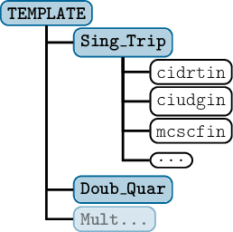
6.21.4 During setup
If you want to set up trajectories for SHARC_COLUMBUS.py, you have to select in the respective setup script the SHARC_LEGACY.py legacy frontend interface.
This is because SHARC_COLUMBUS.py is not yet converted to the SHARC4 format and does not have its own setup routines.
The setup routines are instead in SHARC_LEGACY.py.
After selecting SHARC_LEGACY.py, you will directly be prompted for which of the five legacy interfaces you want to use.
Select SHARC_COLUMBUS.py.
Later during setup, the setup dialogue for SHARC_COLUMBUS.py will be carried out.
During the setup dialogue, you are first queried for the path to the COLUMBUS installation.
You can accept the path from the $COLUMBUS environment variable or enter one manually.
Then you are asked for the scratch directory, where COLUMBUS will store temporary files.
This directory will be deleted after the calculation.
Next, the setup prompts for the path to the COLUMBUS template directory.
The template directory must contain at least one subdirectory for each multiplicity that will be simulated.
Each subdirectory must contain all required input files (control.run, mcscfin, tranin, propin, cidrtin, ciudgin, and optionally cidrtin.* for multiple DRTs).
The script will attempt to match each multiplicity to one of the provided subdirectories automatically.
If necessary, you can manually assign which subdirectory to use for which multiplicity.
Afterward, the script asks for the mapping of mocoef (MO coefficient) files across multiplicities.
Each job (multiplicity-specific subdirectory) can reuse the mocoef file from another job.
In this way, you can, e.g., base all multiplicities’ MRCI computations on the singlet MOs.
If desired, you can choose to copy the entire template directory into each trajectory folder.
By default, it is only linked.
Note that copying will produce a large number of files and directories, especially with many trajectories.
Note that, as a non- SHARC4 interface, the charge given in the template file is not checked against the charges in the dynamics input.
Users must make sure that these are consistent.
You are then asked whether you have an initial MO guess file (e.g., mocoef_mc.init).
While optional, it is strongly recommended to provide one, as CASSCF calculations can otherwise become unstable or very slow.
Finally, you are prompted to enter the amount of memory (in MB) to be made available to COLUMBUS.
If wave function overlaps are needed, the script asks for the path to the overlap executable, the determinant screening threshold, and the number of frozen core orbitals.
If Dyson orbital analysis is also selected, the number of doubly occupied orbitals must be provided.
6.22 BAGEL Interface
Legacy ab initio interface for multi-reference methods in the BAGEL package.
The SHARC– BAGEL interface allows to run SHARC simulations with BAGEL‘s CASSCF, SS-CASPT2, MS-CASPT2, and XMS-CASPT2 functionalities.
The interface is compatible with all multiplicities, but not with symmetry.
Note that separate active spaces are used for each multiplicity.
BAGEL features analytical gradients and nonadiabatic couplings for all of these methods, but no spin-orbit coupings.
Wave function overlaps and Dyson norms can be obtained from the WFOVERLAP code.
QM/MM is not possible, as legacy interfaces cannot handle point charges.
Note that BAGEL does not allow extracting the AO overlap matrix that is required for overlap and Dyson norm calculations; hence, the SHARC– BAGEL interface computes the AO overlaps through PYSCF.
Also note that, currently, it is not recommended to work with MS-CASPT2 gradients and XMS-CASPT2 should always be preferred.
The interface needs two additional input files, a template file for the quantum chemistry (file name is BAGEL.template) and a resource file (BAGEL.resources).
If files QM/archive.<mult>.init are present, they are used to provide an initial orbital guess for the CASSCF calculation of the respective multiplicity.
Note that as a legacy interface, SHARC or parent interfaces cannot control the molecular charge per multiplicity directly, so you need to prepare all BAGEL input with the correct charges in mind.
Note that when running BAGEL, it might be necessary for the user to set $LD_LIBRARY_PATH appropriately, so that all relevant libraries (boost, fabric, …) can be found.
6.22.1 Template file: BAGEL.template
This file contains the specifications for the quantum chemistry calculation. Note that this is not a valid BAGEL input file. The file only contains a number of keywords, given in table 6.33. The actual input for BAGEL will be generated automatically through the interface.
A fully commented template file-with all possible options, a comprehensive descriptions, and some practical hints-is located at $SHARC/../examples/SHARC_BAGEL/BAGEL.template.
We recommend that users start from this template file and modify it appropriately for their calculations.
| Keyword | Description |
| basis | Gives the basis set for all atoms (default svp). It is advisable to always specify a basis set file with absolute path. |
| df_basis | Gives the auxiliary basis set (default: svp-jkfit). It is advisable to always specify a DF basis set file with absolute path. |
| dkh | Activates the (scalar-relativistic) Douglas-Kroll-Hess Hamiltonian. |
| nact | Number of active orbitals. |
| nclosed | Number of closed-shell orbitals. |
| nstate | Number of state-averaging states per multiplicity. |
| method | Can be casscf, caspt2, ms-caspt2, or xms-caspt2. |
| shift | Level shift for CASPT2 (default: 0.0, give float in Hartree). |
| shift_imag | Switches from real to imaginary level shift (use shift to specify the magnitude). |
| orthogonal_basis | Switches on the orthogonal_basis option of BAGEL. Is activated automatically for imaginary level shifts. |
| msmr | Switches on multi-state-multi-reference treatment in CASPT2. Default is single-state-single-reference (SS-SR). |
| maxiter | Iteration limit for energy calculations (SCF, PT2). Default 500. A too high value can slow down the calculation unnecessarily. |
| maxziter | Iteration limit for Z-vector calculations (gradients, NACME). Default 100. A too high value can slow down the calculation unnecessarily. |
| charge | Sets the total charge of the system. Can be either followed by a single integer (then the interface will automatically assign the charges to the multiplicities) or by one charge per multiplicity. |
| frozen | Number of frozen core orbitals for CASPT2 steps. Default is -1, which lets BAGEL automatically decide. |
6.22.2 Resource file: BAGEL.resources
The file BAGEL.resources contains mainly paths (to the BAGEL executables, to the scratch directory, etc.) and other resources, plus settings relevant for wfoverlap.x. This file must reside in the same directory where the interface is started. It uses a simple “keyword argument” syntax. Comments using # and blank lines are possible, the order of keywords is arbitrary. Lines with unknown keywords are ignored, since the interface just searches the file for certain keywords.
The BAGEL interface employs essentially all keywords from Tables 6.3 (except: ngpu), as well as WFOVERLAP keywords from Table 6.4.
Interface-specific keywords are given in Table 6.34.
A fully commented resource file with all possible options and comprehensive descriptions is located in $SHARC/../examples/SHARC_BAGEL/.
| Keyword | Description |
| bagel | Is the path to the BAGEL installation directory. This directory should contain subdirectories bin/ and lib/. Relative and absolute paths, environment variables and can be used. The interface will automatically update the $LD_LIBRARY_PATH. |
| mpi_parallel | If given, the interface will call BAGEL with mpirun -n NCPU, otherwise it will use OpenMP. |
| dipolelevel | Followed by an integer which is either 0, 1, or 2. Controls which dipole moment calculations are skipped by the interface. |
Note that the dipolelevel keyword can have significant impact on the calculation time.
Generally, in CASPT2 calculations, extra computational effort is required for the calculation of state and transition dipole moments.
However, dipole moments have only influence in the dynamics simulations if a laser field is present.
Using the dipolelevel keyword, it is possible to deactivate dipole moment calculations if they are not required.
There are three different settings for dipolelevel:
- dipolelevel=0: The interface will return only dipole moments which can be calculated at no cost (state dipole moments of states where a gradient is calculated; transition dipole moments if nonadiabatic couplings are calculated)
- dipolelevel=1: In addition, the interface will calculate transition dipole moments between S0 and excited singlet states. Use at least this level for the initial condition setup (setup_init.py takes care of this).
- dipolelevel=2: The interface will calculate all state and transition dipole moments
If only energies and dipole moments are calculated, dipolelevel=1 is only slightly more expensive than dipolelevel=0, while dipolelevel=2 increases computation time more strongly.
However, the computation time also depends on whether or not nonadiabatic couplings and gradients are calculated.
Parallelization
The parallel scaling behavior of BAGEL heavily depends on the system (number of atoms, active space, frozen core, …) and on the parallelization mode (MPI or OpenMP).
Hence, it is advisable that the optimal settings (number of cores, parallelization mode) are tested before starting dynamics projects.
Note that the interface can only trivially parallelize BAGEL calculations across several independent multiplicities, but not across multiple gradient or nonadiabatic coupling calculations.
6.22.3 During setup
If you want to set up trajectories for SHARC_BAGEL.py, you have to select in the respective setup script the SHARC_LEGACY.py legacy frontend interface.
This is because SHARC_BAGEL.py is not yet converted to the SHARC4 format and does not have its own setup routines.
The setup routines are instead in SHARC_LEGACY.py.
After selecting SHARC_LEGACY.py, you will directly be prompted for which of the five legacy interfaces you want to use.
Select SHARC_BAGEL.py.
Later during setup, the setup dialogue for SHARC_BAGEL.py will be carried out.
During the setup dialogue, you are first queried for the path to the BAGEL installation.
Then you are asked for the scratch directory, where BAGEL will store temporary files.
This directory will be deleted after the calculation.
Next, the setup prompts for the path to the BAGEL template.
The file is checked for completeness.
It must contain at least the basis set, the density fitting basis, and the number of active and inactive orbitals.
The file also has to contain information about the number of states for state-averaging.
Next, the setup dialogue asks for the dipole level (see above).
Then, the user is asked to set up the initial orbitals.
While optional, it is strongly recommended to provide one, as CASSCF calculations can otherwise become unstable or very slow.
You are then asked for the number of CPU cores and whether to use MPI parallelization.
It is not possible to control the memory used by BAGEL.
In BAGEL, MPI parallelization is more efficient than OpenMP.
If wave function overlaps are needed, the script asks for the path to the overlap executable and the memory for the overlap code.
There is no wave function truncation threshold, because CASSCF wave functions are very efficiently computed with wfoverlap.x.
If Dyson orbital analysis is also selected, the number of doubly occupied orbitals must be provided.
6.23 MOLPRO Interface
Legacy ab initio interface for CASSCF in the MOLPRO package.
The SHARC– MOLPRO interface allows to run SHARC dynamics with MOLPRO‘s CASSCF wave functions.
RASSCF is not supported, since on RASSCF level state-averaging over different multiplicities is not possible.
The interface uses MOLPRO‘s CI program in order to calculate transition dipole moments and spin-orbit couplings.
Gradients and nonadiabatic coupling vectors are calculated using MOLPRO‘s ALASKA code.
In the new version of the interface, overlaps are calculated using the WFOVERLAP code.
Wavefunction phases between the CASSCF and MRCI wave functions are automatically adjusted.
The interface can trivially parallelize the computation of gradients and coupling vectors over several processors.
Execution of parallel MOLPRO binaries is currently not supported.
Important note: It appears that in some cases the sign of the nonadiabatic coupling vectors randomly changes along a trajectory ran with MOLPRO, and that it is not possible to identify this sign change from the MO and CI coefficients.
Hence, propagation with coupling nacdr is currently discouraged for the SHARC– MOLPRO interface.
Alternative possibilities to run SHARC-CASSCF dynamics with nonadiabatic coupling vectors are given by the MOLCAS (section 6.15) and BAGEL (section 6.22) interfaces.
The SHARC– MOLPRO interface needs two additional input files, which should be present in QM/. Those input files are MOLPRO.resources, which contains, e.g., the paths to MOLPRO and the scratch directory, and MOLPRO.template, which is a keyword-argument input file specifying the CASSCF level of theory.
If QM/wf.init is present, it will be used as a MOLPRO wave function file containing the initial MOs.
For calculations with several “jobs” (see below), initial orbitals can also given as QM/wf.<job>.init.
Note that as a legacy interface, SHARC or parent interfaces cannot control the molecular charge per multiplicity directly, so you need to prepare all MOLPRO input with the correct charges in mind.
6.23.1 Template file: MOLPRO.template
The template file is a keyword-argument list file, similar to the template files of most other interfaces.
A fully commented template file with all possible options is located in $SHARC/../examples/SHARC_MOLPRO/.
For simple cases, an example for the template file looks like this:
basis def2-svp
dkho 2                  # Douglas-Kroll second order
occ 14
closed 10
nelec           24
roots           4 0 3
rootpad         1 0 1
This specifies a SA(4S+3T)-CASSCF(4,4)/def2-SVP calculation for 24 electrons.
Note the rootpad keyword, which adds one singlet and one triplet with zero weight to the state-averaging (so technically this is a SA(5S+4T) calculation, but the results are the same as SA(4S+3T)).
These zero-weight states are sometimes useful to improve convergence of CASSCF.
The interface can also be used to perform several independent CASSCF calculations for different multiplicities (e.g., one CASSCF for the neutral states and another one for the ionic states).
In this case, each independent CASSCF calculation is called a “job”.
In the template, most settings can be modified independently for each job.
An example is given here:
# In this way, users can employ custom basis sets
basis_external /path/to/basisset        # no spaces in path allowed
dkho 2
# job 1 for singlet+triplet; job 2 for doublets
jobs 1 2 1
occ 14 13       # for job 1 and 2
closed 11 10    # for job 1 and 2
nelec           24 23 24   # for job 1
nelec           24 23 24   # for job 2
roots           4 0 3   # for job 1
roots           0 2 0   # for job 2
rootpad         1 0 1   # for job 1
rootpad         0 2 0   # for job 2
This template specifies two jobs, where job 1 should be used to compute singlet and triplet states, and job 2 used for doublet states.
Job 1 is a SA(4S+3T)-CASSCF(2,3) computation, with singlets and triplets each having 24 electrons.
Job 2 is a SA(2D)-CASSCF(3,3) computation, with 23 electrons.
Note how for different jobs it is possible to have different active spaces and state-averaging schemes.
However, keep in mind that all states of a given multiplicity are always calculated in the same job (e.g., it is not possible to have one job for S0 and another job for S1 and S2).
It is also possible to do a mixed input, for example having two jobs, but only giving one number after occ or closed.
The interface provides comprehensive error messages during the template check.
Also note the basis_external keyword. It provides a file, whose content is used in the basis set definition (it is inserted verbatim into basis={...} in the MOLPRO input).
It is possible to use the generated input from the Basis Set Exchange Library, but the basis={ and } need to be deleted from the file.
Remember that molpro_input.py cannot create multi-job templates or templates with the basis_external keyword.
6.23.2 Resource file: MOLPRO.resources
The interface requires some additional information beyond the content of QM.in. This information is given in the file MOLPRO.resources, which must reside in the directory where the interface is started. This file uses a simple “keyword argument” syntax. Comments using # and blank lines are possible, the order of keywords is arbitrary. Lines with unknown keywords are ignored, since the interface just searches the file for certain keywords.
The MOLPRO interface employs essentially all keywords from Tables 6.3 (except: ngpu), as well as WFOVERLAP keywords from Table 6.4.
Interface-specific keywords are given in Table 6.35.
A fully commented resource file for this interface with all possible options is located in $SHARC/../examples/SHARC_MOLPRO
Mandatory keywords are the paths to MOLPRO, the scratch directory, and to the WFOVERLAP executable (the latter for overlap, Dyson, or NACDR calculations).
| Keyword | Description |
| molpro | Is followed by a string giving the path to the MOLPRO directory. This directory should contain the executable molpro.exe. Relative and absolute paths, environment variables and can be used. |
| molpro_arguments | Put all command line options for MOLPRO that you want to use, except -W -I -d, because those are set by the interface. In this way, you can run MOLPRO in parallel (on top of running independent jobs in parallel), but note that the ncpu keyword does not take this into account. |
Parallel execution of MOLPRO
In the new version of the SHARC– MOLPRO interface, calculations of multiple independent active spaces (“jobs”), of several gradients, and of several nonadiabatic coupling vectors are automatically parallelized over the given number of CPU cores.
Note that MOLPRO calls can also be parallelized via the molpro_arguments key in the resource file.
6.23.3 Error checking
The interface is written such that the output of MOLPRO is checked for commonly occuring errors, mostly bad convergence in the MCSCF or CP-MCSCF parts. In these cases, the input is adjusted and MOLPRO restarted. This will be done until all calculations are finished or an unrecoverable error is detected.
The interface will try to solve the following error messages:
EXCESSIVE GRADIENT IN CI This error message can occur in the MCSCF part. The calculation is restarted with a P-space threshold (see MOLPRO manual) of 1. If the error remains, the threshold is quadrupled until the calculation converges or the threshold is above 100.
NO CONVERGENCE IN REFERENCE CI The error occurs in the CI part. The calculation is restarted with a P-space threshold (see MOLPRO manual) of 1. If the error remains, the threshold is quadrupled until the calculation converges or the threshold is above 100.
NO CONVERGENCE OF CP-MCSCF This error occurs when solving the linear equations needed for the calculation of MCSCF gradients or nonadiabatic coupling vectors. In this case, the interface finds in the output the value of closest convergence and restarts the calculation with the value found as the new convergence criterion. This ensures that the CP-MCSCF calculation converges, albeit with lower accuracy for this gradient for this time step.
This error check is controlled by two keywords in the MOLPRO.resources file. The interface first tries to converge the CP-MCSCF calculation to gradaccudefault. If this fails, it tries to converge to the best value possible within 900 iterations. gradaccumax defines the worst accuracy accepted by the interface. If a CP-MCSCF calculation cannot be converged below gradaccumax then the interface exits with an error, leading to the abortion of the trajectory.
6.23.4 Things to keep in mind
Initial orbital guess
For CASSCF calculations it is always a good idea to start from converged MOs from a nearby geometry. For the first time step, if a file QM/wf.init is present, the SHARC– MOLPRO interface will take this file for the starting orbitals. In case of multi-job calculations, separate initial orbitals can be provided with files called QM/wf.<job>.init, where <job> is an integer.
In subsequent calculations, the MOs from the previous step will be used (unless the always_orb_init keyword is used).
Basis sets
In order to employ user-defined basis sets, in the template the keyword basis_external, followed by a filename, can be used.
The interface will then take the content of this file and insert it as basis set definition in the MOLPRO input files (i.e., it will add in the input basis={ <content of the file> }.
Note that the filename must not contain spaces.
6.23.5 During setup
If you want to set up trajectories for SHARC_MOLPRO.py, you have to select in the respective setup script the SHARC_LEGACY.py legacy frontend interface.
After selecting SHARC_LEGACY.py, choose SHARC_MOLPRO.py.
Later during setup, the setup dialogue for SHARC_MOLPRO.py will be carried out.
During the setup dialogue, you are first queried for the path to the MOLPRO executable.
Shell variables and can be used and will be expanded when the interface is started.
Next, you are asked for the scratch directory, where MOLPRO will store temporary files.
This directory will be deleted after the calculation, and its validity cannot be checked by the script since you may run the calculations on a different machine.
Then the setup prompts for the path to the MOLPRO.template file.
This file is checked for the following keywords: basis, closed, occ, nelec, and roots.
If a file named MOLPRO.template exists in the working directory and passes this check, you may choose to use it; otherwise, you will be prompted to provide a valid template filename.
Next, the setup dialogue asks for an initial wavefunction guess.
You will be asked whether you have a MOLPRO wavefunction file (e.g. wf.init); if so, you must supply its path.
If not, a warning is issued reminding you that CASSCF calculations may run very long or yield incorrect results without proper starting MOs.
You are then asked to specify the amount of memory available to MOLPRO (in MB) and the number of CPUs to be used by each trajectory.
If wave function overlaps are needed, you will also be prompted for the path to the wfoverlap.x executable.
Note that the MOLPRO interface computes wave function overlaps not only when they are explicitly requested, but also when nonadiabatic coupling vectors are requested, in order to match the wave function phases of the CASSCF wave function (from which the nonadiabatic couplings are computed) and the wave function in the MRCI module (which computes spin-orbit couplings and dipole moments).
Finally, default values for gradient accuracy thresholds (molpro.gradaccudefault, molpro.gradaccumax), number of core orbitals (molpro.ncore), and number of doubly occupied orbitals (molpro.ndocc) are set automatically.
During job preparation, the setup routines write a MOLPRO.resources file into the job directory, containing: the molpro executable path, the scratchdir and savedir locations, gradient accuracy defaults (gradaccudefault, gradaccumax), memory and ncpu settings, and optionally the wfoverlap executable path.
6.23.6 Molpro input generator: molpro_input.py
In order to quickly setup simple inputs for MOLPRO, the SHARC suite contains a small script called molpro_input.py. It can be used to setup single point calculations, optimizations and frequency calculations on the HF, DFT, MP2 and CASSCF level of theory. Of course, MOLPRO has far more capabilities, but these are not covered by molpro_input.py. However, molpro_input.py can also prepare template files which are compatible with the SHARC– MOLPRO interface (MOLPRO.template file).
The script interactively asks the user to specify the calculation and afterwards writes an input file and optionally a run script.
Input
Type of calculation
Choose to either perform a single-point calculation or a minimum optimization (including optionally frequency calculation), to generate a template file, or an optimization of a state crossing. For the template generation, no geometry file is needed, but the script looks for a MOLPRO.input in the same directory and allows to copy the settings.
For single-point calculations, optimizations and frequency calculations, files in MOLDEN format called geom.molden, opt.molden or freq.molden, respectively, are created (containing the orbitals, optimization steps and normal modes, respectively). The file freq.molden can be used to generate initial conditions with wigner.py.
Geometry
Specify the geometry file in xyz format. Number of atoms and total nuclear charge is detected automatically. After the user inputs the total charge, the number of electrons is calculated automatically.
In the case of the generation of a template file, instead only the number of electrons is required.
Non-default atomic masses
If a frequency calculation is requested, the user may modify the mass of specific atoms (e.g. to investigate isotopic effects). In the following menu, the user can add or remove atoms with their mass to a list containing all atoms with non-default masses. Each atom is referred to by its number as in the geometry file. Using the command show the user can display the list of atoms with non-default masses. Typing end confirms the list.
Note that when using the produced MOLDEN file later with wigner.py, the user has to enter the same non-default masses again, since the MOLDEN file does not contain the masses and wigner.py has no way to retrieve these numbers.
Level of theory
Supported are Hartree-Fock (HF), density functional theory (DFT), Møller-Plesset perturbation theory (MP2), equation-of-motion coupled-cluster with singles and doubles (EOM-CCSD) and CASSCF (either single-state or state-averaged). All methods (except EOM-CCSD) are compatible with odd-electron wave functions (molpro_input.py will use the corresponding UHF, UMP2 and UKS keywords in the input file, if necessary).
For template generation, state-average CASSCF is automatically chosen. All methods (except EOM-CCSD) can be combined with optimizations and frequency calculations, however, the frequency calculation is much more efficient with HF or SS-CASSCF.
DFT functional
For DFT calculations, enter a functional and choose whether dispersion correction should be applied. Note that the functional is just a string which is not checked by molpro_input.py.
Basis set
The basis set is just a string which is not checked by molpro_input.py.
CASSCF settings
For CASSCF calculations, enter the number of active electrons and orbitals.
For SS-CASSCF, only the multiplicity needs to be specified. For SA-CASSCF, specify the number of states per multiplicity to be included. Note that MOLPRO allows to average over states with different numbers of electrons. This feature is not supported in molpro_input.py. However, the user can generate a closely-matching input and simply add the missing states to the CASSCF block manually.
For optimizations at SA-CASSCF level, the state to be optimized has to be given. For crossing point optimizations, two states need to be entered. The script automatically detects whether a conical intersection or a crossing between states of different multiplicity is requested and sets up the input accordingly.
EOM-CCSD settings
EOM-CCSD calculations allow to calculate relatively accurate excited-state energies and oscillator strengths from a Hartree-Fock reference, but only for singlet excited states.
The user has to specify the number of states to be calculated. If only one state is requested, the script will setup a regular ground state CCSD calculation, while for more than one states, an EOM-CCSD calculation is setup.
Note that the calculation of transition properties takes twice as long as the energy calculation itself.
Memory
Enter the amount of memory for MOLPRO. Note that values smaller than 50 MB are ignored, and 50 MB are used in this case.
Run script
If requested, the script also generates a simple Bash script (run_molpro.sh) to directly execute MOLPRO. The user has to enter the path to MOLPRO and the path to a suitable (fast) scratch directory.
Note that the scratch directory will be deleted after the calculation, only the wave function file wf will be copied back to the main directory.
6.24 PySCF Interface
Legacy ab initio interface for running CASSCF and PFDT calculations with PYSCF.
The SHARC– PYSCF interface allows to run SHARC dynamics with an implementation of state-averaged CASSCF and PDFT in PYSCF.
The interface can compute energies, dipole moment matrices, gradients, and nonadiabatic coupling vectors.
Spin-orbit couplings, wave function overlaps, or other advanced features are not available.
The interface can only compute singlet states currently.
The interface supports some parallelism, as provided by PYSCF’s OpenMP capabilities, but note that the number of used cores cannot be strictly controlled (some parts of the calculation will use all available cores).
The PDFT implementation requires the installation of PySCF Forge.
With this implementation, the variants MC-PDFT (multi-configurational pair DFT), CMS-PDFT (compressed state multistate PDFT), and L-PDFT (linearized PDFT) are available.
See the Documentation for details and references.
The SHARC– PYSCF interface needs two additional input files, which should be present in QM/. Those input files are PYSCF.resources, which contains, e.g., the paths to PYSCF and the scratch directory, and PYSCF.template, which is a keyword-argument input file specifying the level of theory.
If QM/pyscf.init.chk is present, it will be used for the initial MOs.
Note that as a legacy interface, SHARC or parent interfaces cannot control the molecular charge per multiplicity directly, so you need to prepare all PYSCF input with the correct charges in mind.
6.24.1 Template file: PYSCF.template
This file contains the specifications for the quantum chemistry calculation. Note that this is not a valid BAGEL input file. The file only contains a number of keywords, given in table 6.36. The actual input for BAGEL will be generated automatically through the interface.
A fully commented template file-with all possible options, a comprehensive descriptions, and some practical hints-is located at $SHARC/../examples/SHARC_PYSCF/PYSCF.template.
We recommend that users start from this template file and modify it appropriately for their calculations.
| Keyword | Description |
| basis | (string) Any string that PYSCF recognizes as a basis set. This keyword is mandatory, not giving it results in an error. |
| method | (string) Any one of “casscf”, “l-pdft”, “mc-pdft”, or “cms-pdft”. Default is CASSCF. |
| pdft-functional | (string) Any one of “tpbe” or “ftpbe”. Default is T-PBE. |
| ncas | (int) Number of active orbitals. This keyword is mandatory, not giving it results in an error. |
| nelecas | (int) Numer of active electrons. This keyword is mandatory, not giving it results in an error. |
| roots | (int) Number of states for state-averaging. This keyword is mandatory, not giving it results in an error. |
| charge | (int) Total molecular charge. Default is zero. From the charge and nelecas, the number of inactive electrons is determined (this must be even). Note that for a legacy interface, SHARC or parent interfaces cannot control the molecular charge per multiplicity directly, so the charge must be given in the template. |
| grids-level | (int) A number specifying the DFT quadrature, between 2 and 6. Default is 4. |
| conv-tol | (float) Convergence criterion for CASSCF solver. Default 1e-7. |
| conv-tol-grad | (float) Convergence criterion for CASSCF solver. Default 1e-4. |
| max-stepsize | (float) Step size for CASSCF solver. Default 0.02. |
| max-cycle-macro | (int) Maximum number of macro cycles. Default 50. |
| max-cycle-micro | (int) Maximum number of micro cycles. Default 4. |
| ah-level-shift | (float) Setting for the AH solver of PYSCF. Default 1e-8. |
| ah-conv-tol | (float) Setting for the AH solver of PYSCF. Default 1e-12. |
| ah-max-cycle | (int) Setting for the AH solver of PYSCF. Default 30. |
| ah-lindep | (float) Setting for the AH solver of PYSCF. Default 1e-14. |
| ah-start-tol | (float) Setting for the AH solver of PYSCF. Default 2.5. |
| ah-start-cycle | (int) Setting for the AH solver of PYSCF. Default 3. |
| fix-spin-shift | (float) Necessary shift when using the PYSCF-internal CASSCF solver. Default 0.2. Not used if pyscf-forge is installed. |
| grad-max-cycle | (int) Maximum number of cycles in the coupled-perturbed equations needed for gradients. Default 50. |
| verbose | (int) Print level of the PYSCF output. Default is 3, which gives only sparse output of results. Use 4-6 to obtain more output. The output file PySCF_<job>.log will be located in the directory where the interface runs (this might be located in the scratch directory assigned to SHARC_LEGACY.py). |
6.24.2 Resource file: PYSCF.resources
The file PYSCF.resources contains mainly paths (to the PYSCF executables, to the scratch directory, etc.) and other resources, plus settings relevant for wfoverlap.x. This file must reside in the same directory where the interface is started. It uses a simple “keyword argument” syntax. Comments using # and blank lines are possible, the order of keywords is arbitrary. Lines with unknown keywords are ignored, since the interface just searches the file for certain keywords.
The PYSCF interface employs keywords from Tables 6.3 (scratchdir, savedir, memory, ncpu, always_guess, always_orb_init).
There are no other interface-specific keywords.
A fully commented resource file with all possible options and comprehensive descriptions is located in $SHARC/../examples/SHARC_PYSCF/.
6.24.3 During setup
If you want to set up trajectories for SHARC_PYSCF.py, you have to select in the respective setup script the SHARC_LEGACY.py legacy frontend interface.
After selecting SHARC_LEGACY.py, immediately choose SHARC_PYSCF.py.
The setup dialogue for SHARC_PYSCF.py will then be carried out later during the setup script.
During the setup dialogue, you are first prompted for the scratch directory.
This directory will be used to store the PySCF temporary files and will be deleted after the calculation.
Since you may run the calculation on a different machine, the script cannot verify whether the path is valid, nor will it expand shell variables or during setup (these will be expanded during interface run time).
Next, you are asked for the path to the PYSCF.template file.
If a file named PYSCF.template exists in your working directory, you will be offered to use it; otherwise, you must specify a valid template filename.
This file should contain whatever input directives you require for your PySCF calculation, as the interface will generate the remainder of the input automatically.
You will then be queried about an initial wavefunction guess.
If you have a previous checkpoint file with MOs, you can supply its path; the file will be copied as pyscf.init.chk into the job directory.
If you choose not to provide a guess, a warning reminds you that CASSCF calculations may run very slowly or yield incorrect results without a proper starting wavefunction.
Finally, you must specify the amount of memory (in MB) that PySCF may use.
Currently, the number of CPU cores cannot be set during setup.
When the job is prepared, a file named PYSCF.resources is written into the job directory containing the scratch directory and memory settings.
The specified PYSCF.template is copied into the directory, and-if provided-the initial wavefunction file is also placed there.
6.25 ASE Database Interface
Single child hybrid interface that stores data into an ASE database.
The SHARC– ASE_DB (Atomic Simulation Environment) interface is a single-child hybrid interface that intercepts data from its child interface and stores it into an ASE database.
During interception the data will not be changed and is then directly passed to a parent interface or the SHARC driver.
This interface is particularly useful to generate datasets for training machine learning models.
Available features
The SHARC– ASE_DB interface provides exactly the same set of features as the chosen child interface, without any restrictions.
6.25.1 Template file: ASE_DB.template
The ASE_DB.template file is written in yaml format. Table 6.37 lists the existing keywords.
A fully commented template file for this interface with all possible options is located in $SHARC/../examples/SHARC_ASE_DB/.
| Keyword | Description |
| reference | Specifies the reference SHARC interface that is used to generate the data. Is a dictionary that contains three keys, ïnterface” contains the name of the child interface being used, followed by a list ärgs” that contains arguments which are used to instantiate the child interface, and “kwargs” that contains a dictionary of keyword arguments which are used to instantiate the child interface. |
| props_to_save | Is a list with the names of the properties to be stored in the ASE database. |
| ase_file | Name or path of the ASE database file, if the file already exists the data will be appended. |
| format | Specifies the format of the stored data. There are two options, ßharc” which leaves the data as is, and ßpainn” which converts the data into a format SPaiNN uses. |
| output_steps | Save every nth step to the database. |
6.25.2 During setup
As a hybrid interface, there are some peculiarities when doing a setup with SHARC_ASE_DB.py.
To use SHARC_ASE_DB.py with any child interface, during setup select SHARC_ASE_DB.py.
Immediately after, you will get prompted to provide the ASE_DB.template file, which contain the information of which child interface is desired.
The ASE_DB interface will then instantiate its child, in order to access the child’s feature set and itself returning its feature set to the setup script.
Note that if the child interface is another hybrid interface, then you will get asked for that interface’s template file as well, until all interfaces of the call tree are specified.
The details depend slightly on which hybrid interface you use.
The situation is different if SHARC_ASE_DB.py is not the topmost interface in the call tree.
In that case, the template file of the calling hybrid interface has to specify the ASE_DB interface as a child.
After selecting the interface and its child(ren), at a later point the setup script will start the interface-specific setup dialogue.
However, SHARC_ASE_DB.py itself does not require any settings itself and directly delegates to the child’s interface-specific setup dialogue.
Pay attention to the Setting up child interface notice.
6.26 Umbrella Sampling Interface
Single-child hybrid interface to add various harmonic restraints to a molecule.
The SHARC-umbrella sampling interface allows adding harmonic restraints to any other calculation.
Restraints are possible for distances, angles, dihedrals, and energy gaps.
Multiple restraints are possible.
The sum of all restrain energies is added uniformly to all state energies, and their gradients are added uniformly to all state gradients, for those gradients that were requested by the caller.
If pytorch is installed, it will be used to compute the energies and gradients of all geometrical restraints (distances, angles, dihedrals), but not for energy gaps.
If pytorch is not installed, all restraints are nonetheless available through a custom implementation of energies and forces.
For energy gap restraints, the gradient of both involved states will be added to the set of requested states received from the caller (or of all involved states if more than one energy gap restraint is used).
Available features
The SHARC-umbrella sampling interface provides exactly the same set of features as the chosen child interface, without any restrictions.
6.26.1 Template file: UMBRELLA.template
The interface requires three files in total: a template file in standard SHARC syntax, the restraint file, and the resources file.
Table 6.38 provides the keys for the template file.
| Keyword | Description |
| restraint_file | (string) Path to the file containing the restraint specifications. See below for the format of this file. |
| child-program | (string) Name of the child interface. For interface SHARC_<name>.py, provide the <name> part here. It will be automatically made uppercase. This keyword is required. |
| child-dir | (string) Relative path to the folder containing the input files for the child interface. Default is <NAME>/. |
6.26.2 Restraints file
The restraints file specifies the restraints to add to the potential energy of all states.
The file contains one line per restraint, in the following way:
r   300. kcal/mol angstrom   1.4 angstrom  1 2
a   800. cm-1     degree    90.0 degree    1 2 3
d    75. kj/mol   radian     0.0 radian    1 2 3 4
de   4.6 per      eV         0.3 eV        1 2
Here, column 1 specifies the type of restraint.
The keywords are case-insensitive.
There can be as many lines/restraints as desired, of any type of restraint.
Column 2 specifies the numerical value of the force constant k used in the harmonic restraint.
In principle, this force constant is internally used in terms of units of Hartree energy, Bohr radius, and radians.
To simplify their input, columns 3 and 4 can be used to provide units.
In the example, the force constants are 300 kcal/mol/Å, 800 cm−1/degree, 75 kJ/mol/radian, and 4.6 eV−1.
Here, each unit keyword defines a factor, and the numerical value in column 2 is multiplied by the factor from column 3 and divided by the factor from column 4.
The keywords eh, bohr, radian, one, and per are aliases for a factor of 1.
Other possible keywords are kcal/mol, kj/mol, eV, angstrom, and degree, with the respective conversion factors.
All keywords are case-insensitive.
Columns 5 and 6 specify the position of the minimum of the harmonic restraint, called the reference value below in the equations.
The keywords in column 6 act as multiplicative factors to the numerical value, and all the same keywords can be used.
The keywords in column 6 do not need to be the same as in column 4.
Columns 7 and further ones specify the indices of the atoms or states that are involved in the restraints.
Indices for atoms and for states both start at 1.
For bonds, two indices must be given, and the restraint is invariant under switching of the two indices.
For angles, three indices must be given, where the second index defines the apex atom.
For dihedrals, four indices must be given, in the order in which they are connected.
For energy gaps, two indices must be given, where the second index will be used as the upper state (see equation below, a positive reference energy gap will force the second state to be above the first state).
This choice is made so that “negative” gaps can be sampled, e.g., if one of the states is a singlet and one is a triplet.
Note that the state indices follow standard SHARC state indexing (in the MCH representation, which is the representation that the interfaces work in).
The following energy expressions are used:
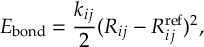
|
(6.12) |
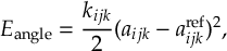
|
(6.13) |
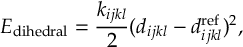
|
(6.14) |
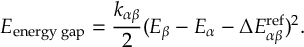
|
(6.15) |
Here, i, j, k, and l are atom indices, α and β are state indices (β is assumed to be the upper state), k is a force constant, and “ref” indicates the chosen center of the bias potential.
6.26.3 Resource file: UMBRELLA.resources
The resource file has only one keyword, as given in Table 6.39.
| Keyword | Description |
| scratchdir | (string) Path to the scratch directory. This will be used to override the scratch directory of the child, as is customary for hybrid interfaces (likewise, if SHARC_UMBRELLA.py is called from a hybrid parent interface, then the scratchdir from UMBRELLA.resources will be ignored). |
6.26.4 During setup
As a hybrid interface, there are some peculiarities when doing a setup with SHARC_UMBRELLA.py.
To use SHARC_UMBRELLA.py, select it directly in your setup script.
Immediately, you will be prompted for the path to your UMBRELLA.template file, which tells the interface which child program to invoke (plus other details).
If your child is itself a hybrid interface, you will then be asked for that interface’s own template file, and so on down the call tree.
After reading the template, you will be asked if you already have an UMBRELLA.resources file.
If so, supply its path here; otherwise it will remain absent (but SHARC_UMBRELLA.py does not have many resource options).
Next you will see a Setting up child interface notice.
At this point, SHARC_UMBRELLA.py hands off to the child interface’s own setup dialogue.
6.27 Droplet Potential Interface
Single-child hybrid interface to add droplet and tether potentials/forces to a condensed system.
The SHARC-droplet potential interface allows various positional harmonic restraints to any other calculations.
There are three main applications, all mainly intended for large systems (e.g., with QM/MM).
First, a droplet potential is a flat-bottom harmonic potential affecting all atoms, in order to avoid that a nanodroplet of solvent evaporates.
Second, a tether potential is a flat-bottom harmonic potential affecting the solute, in order to avoid that the solute diffuses to the edge of the droplet.
Third, one can use general positional harmonic restraints to anchor some atoms to a position, e.g., to mimic the effect of a larger surrounding or replicate “QM/MM/MM” schemes.
The sum of all restrain energies is added uniformly to all state energies, and their gradients are added uniformly to all state gradients, for those gradients that were requested by the caller.
The functional form of the potential is
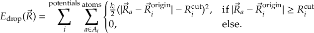
|
(6.16) |
Available features
The SHARC-droplet potential interface provides exactly the same set of features as the chosen child interface.
The only exception is that the droplet potential interface does not support point charges, and so typically must be used as the top-level interface, e.g., above the QM/MM interface.
6.27.1 Template file: DROPLET.template
The template file for the droplet interface is in YAML format.
An example is shown here:
child:
  name: QMMM
  interface: QMMM
  dir: QMMM
  args: []
  kwargs: {}
droplet_potentials:
- name: droplet1
  Rcut: 7.1570497149398085
  k: 3.6104814718939656e-05
  origin: [0.0, 0.0, 0.0]
  atoms: all
- name: droplet2
  Rcut: 4.0
  k: 6.0e-05
  origin: com
  atoms: [1,2,3,4]
The template file is automatically generated during setup.
Note that the names of the potentials have no effect.
Note the special keywords all for the atoms entry and com for the origin entry.
The former simply selects all atoms, whereas the latter sets the origin based on the center of mass of the selected atoms during the first time step/calculation.
The names of the individual potentials are only used for some warning/error messages and do not affect the calculation.
6.27.2 Resource file: DROPLET.resources
The resource file has only one keyword, as given in Table 6.40.
| Keyword | Description |
| scratchdir | (string) Path to the scratch directory. This will be used to override the scratch directory of the child, as is customary for hybrid interfaces (likewise, if SHARC_DROPLET.py is called from a hybrid parent interface, then the scratchdir from DROPLET.resources will be ignored). |
6.27.3 During setup
As a hybrid interface, there are some peculiarities when doing a setup with SHARC_DROPLET.py.
To use SHARC_DROPLET.py, select it directly in your setup script.
Immediately, you will be prompted for which child interface to invoke.
If your child is itself a hybrid interface, you will then be asked for that interface’s own template file, and so on down the call tree.
Later during setup, you will be asked if you already have an UMBRELLA.resources file.
If so, supply its path here; otherwise it will remain absent (but SHARC_DROPLET.py does not have many resource options).
Next, you will be able to specify the parameters for your droplet potentials.
The parameters can either be set up automatically or manually.
For automatic setup, the parameters are obtained from:
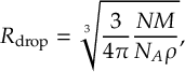
|
(6.17) |
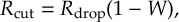
|
(6.18) |
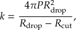
|
(6.19) |
where N is number of molecules, M is molar mass, NA is Avogadro’s constant, ρ is density, W is defining the flat-bottom part, and P is pressure.
These equations first compute the radius of a sphere of N molecules with molar mass M and density ρ, then use the W parameter (W=1 is a hard wall, W=0 is a harmonic potential without flat bottom) to compute the cutoff radius.
Finally, the force constant is computed from the pressure P at the surface of the sphere.
As last part of the setup of the droplet interface, you will see a Setting up child interface notice.
At this point, SHARC_DROPLET.py hands off to the child interface’s own setup dialogue.
6.28 Classical Path Approximation (CPA) Interface
Single-child hybrid interface to copy the ground state gradient to every state.
The SHARC– CPA single-child hybrid interface allows to run SHARC simulations within the Classical Path Approximation (CPA)[84,[85] dynamics, i.e., the effect of the electron dynamics on the nuclear motion (electron-nuclear back reaction) is neglected. In other words, the nuclear forces driving the dynamics of the nuclei always correspond to the ground-state forces, regardless of what the electron dynamics does.
Usually, when CPA is employed, velocity rescaling upon hopping is replaced by scaling the transition probability of hops upward in energy (i.e., from lower state to higher state) by a Boltzmann scaling factor, thus ensuring detailed balance, see Ref. [84].
To do so in SHARC it is necessary to specify the boltzmann_hop and boltzmann_temperature temperature_value keywords in the input file (section 4.1).
Usually, if this option is activated, no velocity rescaling should be employed [84] (ekincorrect none). If boltzmann_hop is found in the input and ekincorrect is not set to none then SHARC enforces ekincorrect none.
Note that with the CPA interface, total energy will not be conserved, unless the trajectory runs in the ground state.
We recommend to turn off the corresponding check in diagnostics.py (by setting the total energy thresholds to very large numbers).
Available features
The single-child SHARC– CPA interface provides exactly the same set of features as the chosen child interface.
The only exception is that only the ground-state nuclear gradients are requested to the child-interface, regardless of its capability to additionally provide the excited-state ones. The same ground-state gradients are the used for each active state of the dynamics, including the excited states.
The interface requires a template file (CPA.template) and optionally a resource file (CPA.resources)
6.28.1 Template file: CPA.template
The CPA.template file is written in yaml format. Table 6.41 lists the existing keywords.
| Keyword | Description | |||
| Keyword | Description |
| scratchdir | (string) Path to the scratch directory. This will be used to overwrite the scratch directory of the child, as is customary for hybrid interfaces (likewise, if SHARC_CPA.py is called from a hybrid parent interface, then the scratchdir from CPA.resources will be ignored). |
If CPA.resources is not specified then scratchdir will be set according to the default value (see Table 6.3).
6.28.3 During setup
As a hybrid interface, there are some peculiarities when doing a setup with SHARC_CPA.py.
To use SHARC_CPA.py with any child interface, during setup select SHARC_CPA.py.
Immediately after, you will get prompted to provide the CPA.template file, which contains the information of which child interface is desired. The interface will try to locate it in the current folder where the setup scripts is run, if it is not found then the user will be asked to provide the path to it.
If CPA.resources is also found it will be used, otherwise the default options will be assumed.
The CPA interface will then instantiate its child, in order to access the child’s feature set and itself returning its feature set to the setup script.
Note that if the child interface is another hybrid interface, then you will get asked for that interface’s template file as well, until all interfaces of the call tree are specified.
The details depend slightly on which hybrid interfaces you use.
After selecting the interface and its child, at a later point the setup script will start the interface-specific setup dialogue.
However, SHARC_CPA.py itself does not require any settings itself and directly delegates to the child’s interface-specific setup dialogue.
Pay attention to the Setting up child interface notice.
6.29 Numerical Differentiation Interface
Single-child hybrid interface (with clones of the same child) for finite differences numerical gradients and nonadiabatic coupling vectors.
The SHARC-numerical differentiation interface can compute gradients, nonadiabatic coupling vectors, dipole moment derivatives, and spin-orbit coupling derivatives for any other interface that can provide energies, wave function overlaps, dipole moments, and spin-orbit couplings, respectively.
Currently, the interface is based on central differences evaluated in Cartesian coordinates, using uniform displacements for all atoms and directions.
The interface can do the derivatives in two different ways (numdiff_representation), either using the adiabatic quantities directly, or using wave function overlaps to diabatize the quantities and computing their derivatives.
The latter option is slightly more expensive but more numerically stable if electronic state crossings occur close to the reference geometry.
For ease of reference, we provide the essential equations here.
Adiabatic central differences are evaluated as:
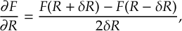 |
(6.20) |
where F is a matrix element of the Hamiltonian, overlap, or dipole matrices.
For the quad-step central differences, the equation is instead:
 |
(6.21) |
For diabatic central differences, the equation is:
 |
(6.22) |
where the entire Hamiltonian or dipole matrices F are transformed before computing the derivative.
Note that S(R, R+δR)=S(R+δR, R)†.
In the diabatic mode, the nonadiabatic couplings are computed as the energy-gap-scaled off-diagonal elements of the derivatives of the diabatic Hamiltonian (i.e., [1/(∆E)][(∂H)/(∂R)]):
 |
(6.23) |
Note that fast child interfaces will generally be run in non-persistent mode (i.e., with file I/O).
Hence, numerical differences of fast interfaces will be slower than expected.
These restrictions arise because SHARC_NUMDIFF.py manipulates the save directory of its child, but hybrid children would have an unpredictable save directory structure and fast interfaces in persistent mode do not write save directories.
Available features
The SHARC-numerical differentiation interface provides features that depend on the features of the child as well as on the numdiff_representation and whitelist options (more details below).
Briefly, if the child can provide energies, then SHARC_NUMDIFF.py can provide gradients.
If the child provides energies and overlaps, SHARC_NUMDIFF.py can provide nonadiabatic coupling vectors.
If the child provides dipole moments or spin-orbit couplings, their respective derivatives are available from SHARC_NUMDIFF.py.
If numdiff_representation is set to diabatic, then all four types of derivatives also require overlaps from the child.
If any of the four quantities would also be available from the child directly, then whitelist can be used to use the quantities from the child rather than from numerical differentiation.
Any request besides gradients, nonadiabatic coupling vectors, dipole moment derivatives, and spin-orbit coupling derivatives is completely delegated to the child interface (for the reference geometry).
Hence, the feature set of SHARC_NUMDIFF.py is the feature set of the child, plus those derivatives that can be computed.
Note that SHARC_NUMDIFF.py does not accept point charges, so it cannot serve as QM interface in QM/MM calculations.
6.29.1 Template file: NUMDIFF.template
The interface requires two input files.
The possible options for the template file are given in Table 6.43.
The file follows standard keyword argument syntax, as in other interfaces.
| Keyword | Description |
| qm-program | (string) Name of the child interface. For interface SHARC_<name>.py, provide the <name> part here. It will be automatically made uppercase. Note that SHARC_NUMDIFF.py formally uses multiple children, but they are clones (all share the same settings), so only one child needs to be specified. This keyword is required. |
| qm-dir | (string) Relative path to the folder containing the input files for the child interface. This keyword is required. |
| numdiff_method | (string) Specifies the numerical differentiation scheme. Currently, options are central-diff (the default) and central-quad. The default uses two displacements per degree of freedom, the second option uses twice as much. See Equations (6.20) and (6.21). |
| numdiff_representation | (string) Specifies the electronic representation for differentiating. Currently, options are adiabatic (the default) and diabatic. The first option uses the adiabatic quantities of the displaced geometries directly, whereas the second option diabatizes them using the overlaps between reference geometry and displaced geometry. This adds the cost of overlap calculations at all displacements, but leads to more accurate derivatives. See Equation (6.22). |
| numdiff_stepsize | (float) The numerical Cartesian displacement in Bohrs. Default is 0.01. For central-quad, additional displacements of twice that value are done. |
| whitelist | (one or more strings) The requests specified here are delegated to the reference child, if it can provide them. Possible options are grad, nacdr, dmdr, and socdr. Note that an empty list is not possible, if you do not want any white-listed requests, remove the whitelist command. |
6.29.2 Resource file: NUMDIFF.resources
The resource file has only few keywords, as given in Table 6.44.
A few remarks on how the children are run.
In all cases, the reference child is run first.
By default, it uses whatever number of CPU cores is specified in its resource file.
If use_all_cores_for_ref is true, the reference child will use all CPU cores available to SHARC_NUMDIFF.py instead.
After the reference child is finished, SHARC_NUMDIFF.py evaluates whether displacement calculations have to be carried out, depending on (i) the current requests, (ii) the whitelist, and (iii) the available features of the child.
If grad, nacdr, dmdr, or socdr are requested and not white-listed and available from the child, they will be computed numerically.
Only then the displaced children will be set up and run, distributed over the number of CPU cores available to SHARC_NUMDIFF.py.
Each displaced child will use as many CPU cores as specified in the child’s resource file.
| Keyword | Description |
| scratchdir | (string) Path to the scratch directory. This will be used to host the scratch directories of all children (reference and displacements), i.e., SHARC_NUMDIFF.py will overwrite the scratch directories of all children (likewise, if SHARC_NUMDIFF.py is called from a hybrid parent interface, then the scratchdir from NUMDIFF.resources will be ignored). |
| ncpu | (int) The number of CPU cores used to run the calculation of the reference and displaced children. Note that the reference child is always run first. Only the displacement children are run in parallel. |
| use_all_cores_for_ref | (bool) Use all CPU cores as available to SHARC_NUMDIFF.py for the reference child. |
6.29.3 During setup
As a hybrid interface, there are some peculiarities when doing a setup with SHARC_NUMDIFF.py.
To use it, select SHARC_NUMDIFF.py directly in your setup script.
You will then immediately be prompted for the path to your NUMDIFF.template file, which tells the interface which underlying QM program to invoke and how to perform the numerical differentiation.
SHARC_NUMDIFF.py will then instantiate its child and query it for its feature set.
Based on that feature set and the settings in the template file, the SHARC_NUMDIFF.py interface automatically composes its own feature set, which is returned to the setup script.
At a later point during setup, the interface-specific setup dialogue is started.
SHARC_NUMDIFF.py will ask for the number of CPU cores and the scratch directory to be used.
Subsequently, the interface-specific setup dialogue of the child is launched (indicated by Setting up QM‑interface).
6.30 QM/MM Interface
Multi-child hybrid interface for QM/MM calculations using electrostatic embedding and link atoms.
The SHARC-QM/MM interface implements
 |
(6.24) |
Here, EQM(QM; MMpc) is the QM energy of the QM region, including its interaction with the MM point charges.
EMM(QM’+MM) is the MM energy of the full system, with QM region point charges set to zero.
EMM(QM’) is the MM energy of the QM region alone, also with QM region point charges set to zero.
Setting the QM region point charges to zero at the MM level prevents double-counting Coulomb interactions, which are already accounted for in the QM calculation.
Within the interface, the three energy contributions from Equation (6.24) are computed in three independent calls to three child interfaces.
These are called the QM, MMS, and MML children, in the order given in the equation.
The interface also supports link atoms, i.e., bonds between a QM and an MM atom.
To make this work, the connectivity table has to be included in the QMMM.table input file (see below).
The link atom scheme[122] is treated as follows in the QM calculation.
All QM atoms are kept, all MM atoms bonded to QM atoms are replaced by hydrogen.
The position of the hydrogen (cap) atoms is defined by the positions of the QM and bonded MM atoms, so the cap atoms do not provide independent degrees of freedom.
The point charge of the bonded MM atom is set to zero, its charge is distributed evenly over all its bonding partners that are MM atoms.
Note that the charge and multiplicity specified in input, QM.in, and other input files is directly passed to the QM interface without any check.
In other words, the MM region is assumed to have charge 0 and singlet multiplicity for the purposes of determining the charge and multiplicity of the QM region.
Available features
The SHARC-QM/MM interface provides features that depend on the features of the QM and MM child interfaces.
For electrostatic embedding (which is currently the only option), the QM interface must have the point_charges feature, i.e., it needs to be able to receive point charges and include them in the QM calculation.
Likewise, the MM interface needs to have the multipolar_fit feature, i.e., it needs to be able to provide partial charges/multipoles for the MM state.
If these features are available, then the QM/MM interface will provide energies and/or gradients if they are available from both the QM and MM interfaces.
All other features are inherited from the QM interface.
The QM/MM interface does not provide the point_charges feature, so it is currently not possible to do nested QM/QM/MM or QM/MM/MM calculations.
6.30.1 Template file: QMMM.template
The interface requires two input files.
The possible options for the template file are given in Table 6.45.
The file follows standard keyword argument syntax, as in other interfaces.
| Keyword | Description |
| qmmm_table | (string) Path to the QMMM.table file containing the connectivity and QM/MM type information. See Section 6.30.3. |
| qm-program | (string) Name of the QM child interface. For interface SHARC_<name>.py, provide the <name> part here. It will be automatically made uppercase. This keyword is required. |
| mm-program | (string) Name of the MM child interface. Note that the MML and MMS children use the same interface class. This keyword is required. |
| embedding | (string) Selects the type of embedding. Currently, only subtractive is allowed (the default). |
| qm-dir | (string) Relative path to the folder containing the input files for the QM child interface. This keyword is required. |
| mml-dir | (string) Relative path to the folder containing the input files for the MML child interface. Default is MML. |
| mms-dir | (string) Relative path to the folder containing the input files for the MMS child interface. Default is MMS. |
| mm_dipole | (bool) If false (the default), then the dipole moments returned by the QM/MM interface are those of the QM interface. If true, then the dipole moment induced by the distribution of MM charges is added to the diagonal of the dipole matrix. |
6.30.2 Resource file: QMMM.resources
This file is currently not used.
6.30.3 Connectivity and QM/MM type file: QMMM.table
This file specifies the connectivity/topology of the system and assigns each atom to either the QM or MM region.
An example file is shown here.
qm  O    2
qm  C    3 4            1
qm  H                   2
qm  C    5 6 7          2
qm  H                   4
qm  H                   4
mm  C    8 9 10         4
mm  H                   7
mm  H                   7
mm  C    11 12 13       7
mm  H                   10
mm  H                   10
mm  H                   10
mm  O    15 16
mm  H                   14
mm  H                   14
The file specifies a OHC-CH2-CH2-CH3 + H2O system (butanal plus one water), where the OHC-CH2 group is in the QM region.
6.30.4 During setup
As a hybrid interface, there are some peculiarities when doing a setup with SHARC_QMMM.py.
To use it, select SHARC_QMMM.py directly in your setup script.
You will then immediately be prompted for the path to your QMMM.template file, which tells the interface which underlying QM and MM interfaces to invoke.
SHARC_QMMM.py will then instantiate its children and query them for their feature set.
Based on these feature sets, the SHARC_QMMM.py interface automatically composes its own feature set, which is returned to the setup script.
At a later point during setup, the interface-specific setup dialogue is started.
SHARC_QMMM.py will ask for a resource file, which will be copied if given.
Subsequently, the interface-specific setup dialogues of the children are launched sequentially (indicated by Setting up QM-interface, Setting up MML-interface (whole system), and for subtractive QM/MM schemes also Setting up MMS-interface (qm system)).
6.31 ECI Interface
Multi-child hybrid interface for excitonic Hartree-Fock and excitonic configuration interaction (EHF/ECI) calculations.
The SHARC-ECI interface (SHARC_ECI.py) implements the ab-initio exciton-like theory for the efficient calculation of ground and excited electronic states of multichromophoric systems, described in the references [123] and [124].
6.31.1 Theory and implementation
The ECI method works as follows, in roughly three steps.
These steps assume that the multichromophoric system is divided into fragments (also called chromophores or sites) that share no atoms (i.e., disjoint fragments).
Site-state calculations
In the first step, SHARC_ECI.py conducts a single-point calculation (so-called site state calculations, SSCs) of the desired number of states (of various multiplicities and charges) for each individual site, with embedding point charges placed on the positions of the nuclei of all other sites.
This gives the set of so-called site states.
One feature of the ECI method is that it is agnostic of the precise electronic-structure ansatz used in the SSC, i.e., the site states can be calculated with any level of theory.
Hence, SHARC_ECI.py performs the SSCs via its SSC children-(some of) the ab-initio interfaces of SHARC.
Building the ECI basis
In the second step, SHARC_ECI.py constructs the so-called excitonic basis-a basis of antisymmetrized products of the site states.
Herein, unlike in conventional exciton models, one can have antisymmetrized products of different kinds-the product of all site ground states (GS product), the products where a single site is in an excited state and all others in the ground state (local excitations, LEs), and the products with an arbitrary number of excited site states (multilocal excitations, MLEs: double-local excitations, DLEs; triple-local excitations, TLEs; …).
Which type of the products will be included in the basis is controlled by specifying the ECI expansion (EHF, ECIS, ECISD,…), where the GS product plays role of excitonic “HF configuration”, LEs play role of excitonic ßingles”, DLEs of excitonic “doubles”, etc.
Note that this does not mean that, e.g., all LEs are electronically singly-excited configurations.
If the excited site state present in an LE is a doubly-excited state itself, the LE will be a doubly-excited configuration (but still an excitonic ßingle”).
Also, this does not mean that the products are individual Slater determinants, but rather correlated configurations, if the site states themselves are.
In this sense, the excitonic basis in ECI is nominally build in the analogous way the CI basis is build: the ground site states are multiplied to give the GS product, and then all desired (M)LEs are generated by exchanging a certain number (one for LEs, two for DLEs) of ground site states in the GS product with excited site states provided for particular fragments in the SSC.
However, the ECI interface is not restricted only to the GS product as the äufbau” one (i.e., the one on which ground-to-excited site state replacements will be done to create LEs and MLEs), but it allows the definition of multiple aufbau site states per fragment, which then give rise to multiple aufbau products, in an each-by-each-multiplication fashion.
Moreover, different aufbau site states of a single fragment can even have different charges (e.g. S0 of neutral fragment, and D0 of fragment’s cation).
Even excited site states can be defined as aufbau site states.
The (M)LEs are then created by replacing a certain number of aufbau site states from each aufbau product with non-aufbau site states of the same charge but not necessarily of the same multiplicity.
For example, in a two-chromophoric system, if only the S0 site states of both fragments are defined as the aufbau site states, only the \ketS0S0 product will be the aufbau product (in this case matching with the GS product).
Then, if each chromophore has S1, T1, D0+, D0−, D1+ and D1− non-aufbau site states provided in the SSCs, and the ECIS expansion is requested, the constructed non-aufbau products will be: \ketS1S0, \ketS0S1, \ketT1S0 and \ketS0T1.
The charge-transfer (CT) products \ketD0+D0− and \ketD0−D0+ will not be constructed, as this would require changing the fragments’ charges.
These products can be constructed by setting all S0, D0+ and D0− site states as the aufbau ones for both fragments.
In this case, the aufbau products will be \ketS0S0, \ketS0D0+, \ketS0D0−, \ketD0+S0, \ketD0−S0, \ketD0+D0− and \ketD0−D0+.
Depending on the specified full-system charge, the interface will take either only \ketS0S0, \ketD0+D0− and \ketD0−D0+ for charge 0, or \ketS0D0+ and \ketD0+S0 for charge 1, or \ketS0D0− and \ketD0−S0 for charge −1.
Then, for charge 0 and an ECIS expansion, the \ketS0S0 aufbau product will give \ketS1S0, \ketS0S1, \ketT1S0 and \ketS0T1 LEs, the \ketD0+D0− will give \ketD1+D0− and \ketD0+D1− LEs, while \ketD0−D0+ will give \ketD1−D0+ and \ketD0−D1+ LEs.
Note that the products (both aufbau or non-aufbau) actually contain the site states with well-defined site-specific S and MS value. In this sense, \ketD0+D0− above is not a single product but rather a symbolic representation of a set of four products, having four combinations of MS values of the two doublet site states: (+\sfrac12,+\sfrac12), (+\sfrac12,−\sfrac12), (−\sfrac12,+\sfrac12) and (−\sfrac12,−\sfrac12).
After all products are generated, the interface will take only those having the total MS value equal to the S value of the specified full-system multiplicity (0 for singlets, \sfrac12 for doublets, 1 for triplets, etc.).
For example, for full-system singlet spin, the interface will take \ketDx+Dy− products only with (+\sfrac12,−\sfrac12) and (−\sfrac12,+\sfrac12) combinations of MS values, while for triplets it will take only (+\sfrac12,+\sfrac12).
Similarly, for full-system triplet spin, only \ketT1S0 with T1 site state having MS=1 will be taken, etc.
However, such products are not necessarily eigenfunctions of the full-system spin.
For example, for singlet spin, \ketS1S0 LE is a singlet configuration, but \ketD0+D0− with either (+\sfrac12,−\sfrac12) or (−\sfrac12,+\sfrac12) is not.
In this case, the singlet function is a linear combination [1/(√2)][(+\sfrac12,−\sfrac12)−(−\sfrac12,+\sfrac12)].
The less obvious example would be \ketD0+T1, which for the full-system doublet spin is a linear combination [1/3][√6(−\sfrac12,+1)−√3(\sfrac12,0)].
These spin-adapted products are called excitonic configuration state functions (ECSFs) and the interface will generate them automatically by diagonalization of the full-system spin operator.
The raw antisymmetrized products are then referred to as excitonic Slater determinants (ESDs), in analogy with the CI method and Slater determinants.
Construction of the ECI Hamiltonian
In the third step, the ECI Hamiltonian matrix of the full system is evaluated for each multiplicity (and MS=S) in the excitonic basis of ESDs.
This is done within the strong orthogonality assumption (SOA).
To construct the ECI Hamiltonian, one needs only two ïngredients” from the each site: the site energies and the site density matrices, which are obtained from the SSC children.
It is important to note that the couplings between the ESDs where the two site states of a fragment differ in the charge are currently neglected, as the underlying theory is under development.
An example for this would be the couplings between an LE and a CT product, e.g., \melS1S0∧HD0+D0−.
The Hamiltonian is then rotated to the basis of ECSFs, and the full-system states are obtained by diagonalization of the ECI Hamiltonian for each full-system multiplicity.
EHF embedding
Importantly, before the SSCs, SHARC_ECI.py can determine the optimal embedding point charges of all atoms of all fragments via the excitonic Hartree-Fock (EHF) method [123].
The EHF algorithm involves iterative ground-state calculations on each fragment with the ground-state RESP point charges of other all fragments placed in the surroundings, followed by the RESP fit of the obtained ground-state densities, until all RESP charges stop changing.
The ground-state calculations and the RESP fits are done via the EHF children of SHARC_ECI.py.
Such obtained charges should minimize the energy of the GS product, just like the optimal orbitals in HF minimize the energy of a Slater determinant.
However, SHARC_ECI.py also has some other options to utilize non-optimal embedding charges in various ways, in order to reduce computational cost (see below in Section 6.31.3).
Note that the EHF part of the SHARC_ECI.py run will not calculate the EHF energy of the system, but will only find the optimal embedding charges (i.e., despite its name, it is an excitonic analogue of SCF rather than HF).
The EHF energy will be calculated later when building the ECI Hamiltonian.
Available features
The SHARC_ECI.py currently provides only the h, dm, mol and point_charges features.
It requires from its EHF children only the multipolar_fit and point_charges.
From the SSC children, it always requires the h, mol, density_matrices and point_charges features, regardless of the requests given to it.
Limitations
The current theoretical framework and implementation entail a few consequences:
- Despite the ECI method being agnostic to the SSC ansatz, the site states can currently only be calculated on CIS/TD-DFT level with Gaussian or on CASSCF level with OpenMolcas, since only SHARC_GAUSSIAN.py and SHARC_MOLCAS.py have the density_matrices feature.
- In order for the method to work accurately, sites can interact strongly but should not be too close in space (e.g., covalently bonded), as this will break the SOA.
The method is supposed to work well for supramolecular aggregates, metal complexes with no low-lying metal-centered excitations, and other similar systems. - Regardless of the system, the method will not diverge in the region of overlapping sites, due to the SOA.
Thus, the method should not currently be used to perform scans (that include close-site region), optimizations, or molecular dynamics.
It is currently primarily intended for the spectroscopic calculations on the systems described in the previous bullet. - Even if the sites might be sufficiently far apart, some of the calculated site states might penetrate the regions of other sites (e.g., Rydberg states) and thus break SOA.
Hence, SHARC_ECI.py will expel those site states prior to the construction of the ECI basis [123].
We intent to overcome these limitations in future releases of SHARC.
6.31.2 QM directory of ECI interface
The QM directory of SHARC_ECI.py has to contain a template file (Section 6.31.3), a resources file (Section 6.31.4), and a directory per child containing its input files.
As mentioned above, SHARC_ECI.py has two types of children-EHF and SSC children.
An EHF child is an interface used to calculate the ground state of a single fragment for a single full-system charge during the EHF procedure.
An SSC child is an interface used to calculate all the (ground and excited) site states for a single fragment and a single charge for a single full-system charge.
All fragments are given a label in ECI.template (see Section 6.31.3).
The names of the QM directories of the EHF children have to be <label>_embedding_Z<Z>, where <Z> is the full-system charge.
The names of the QM directories of the SSC children have to be <label>_z<z>_Z<Z>, where <z> is the fragment charge and <Z> is again the full-system charge.
The template file, the resources file and the structure of the standard output of SHARC_ECI.py will be illustrated in following subsections on an example of an ECI calculation of 6 neutral singlet and 6 neutral triplet states of a system containing two BODIPY chromophores connected via C-H… F hydrogen bond.
Donor is labeled BD and the acceptor BA, while the site states are calculated on TD-ωB97xD/def2svp level with SHARC_GAUSSIAN.py.
The example can be found in $SHARC/../examples/SHARC_ECI.
Since in this case we calculate only full-system neutral states while having site states of BD with charges 0 and 1 and site states of BA with charges 0 and −1 (see below in Section 6.31.3), the QM directory of SHARC_ECI.py in this case contains BD_embedding_Z0, BA_embedding_Z0, BD_z0_Z0, BD_z1_Z0, BA_z0_Z0 and BA_z-1_Z0 children QM subdirectories.
Also, since each child is a SHARC-GAUSSIAN interface (also see in Section 6.31.3), each of these subdirectories contains the only two input files of SHARC_GAUSSIAN.py: GAUSSIAN.template and GAUSSIAN.resources.
6.31.3 Template file: ECI.template
The example below shows a template file of SHARC_ECI.py in yaml format for the aforementioned BD–BA system.
---
fragments:
    BD:
        atoms: 0-20
        aufbau_site_states: [{Z: 0, M: 1, N: 1},{Z: 1, M: 2, N: 1}]
        EHF:
            interface : GAUSSIAN
            embedding_site_state:
                0: {Z: 0, M: 1, N: 1}
            guess: true
            write: true
            max_cycles: 10
            forced: false
            tQ: 0.01
        SSC:
            interface: GAUSSIAN
            data: w
            states:
                0: [2, 0, 1]
                1: [0, 1, 0]
    BA:
        atoms: 21-41
        aufbau_site_states: [{Z: 0, M: 1, N: 1}, {Z: -1, M: 2, N: 1}]
        EHF:
            interface : GAUSSIAN
            embedding_site_state:
                0: {Z: 0, M: 1, N: 1}
            guess: true
            write: true
            max_cycles: 10
            forced: false
            tQ: 0.01
        SSC:
            interface: GAUSSIAN
            data: w
            states:
                0: [2, 0, 1]
                -1: [0, 1, 0]
calculation:
    tO: 0.90
    RI:
        active: true
        Jauxbasis: def2svpjkfit
        Kauxbasis: def2svpjkfit
        tS: 1.e-4
        tC: 1.e-3
        chunksize: -1
    excitonic_basis:
        ECI:
            0: true
            1: all
            2: all
    active_integrals:
        J:
            '(0,0)': [ [BD, BA] ]
            '(0,1)': [ [BD, BA] ]
            '(0,2)': [ [BD, BA] ]
        K:
            '(0,0)': [ [BD, BA] ]
            '(0,1)': [ [BD, BA] ]
            '(0,2)': [ [BD, BA] ]
The top-level dictionary allows only two keys, fragments and calculation.
The fragments is mandatory (no default value), while calculation is not mandatory (see below for the defaults).
The yaml file is generally organized as a hierarchical dictionary.
The following paragraphs specify the syntax and functionality of all the relevant keys.
fragments
The fragments dictionary has to have as many items as there are fragments in the system (in this example case, two).
The minimal number of fragments is one.
The key for each fragment is an arbitrary label of the fragment (in this case, BD and BA).
Note that every fragment must have a unique label.
The dictionary given for each fragment specifies everything related to this fragment in the context of the entire ECI calculation.
fragments: <label>
For each fragment, the following entries must be present: atoms, aufbau_site_states, EHF, and SSC.
fragments: <label>: atoms
The atoms entry specifies the atoms of the full system that belong to this fragment, and is mandatory.
It can be given as a range (e.g., 0-20), or a comma-delimited sequence (e.g., 0,2,5,13), or a combination of the two (e.g., 0-10,15,17,20-22).
The indexation is with respect to the atom ordering given in the QM.in object of the SHARC-ECI interface, and starts with zero.
fragments: <label>: aufbau_site_states
The aufbau_site_states is an arbitrarily long list of aufbau site states of a fragment, and is mandatory.
Each aufbau site state in the list is given as a dictionary with keys: Z – the charge of the state, M – the multiplicity of the state, and N – the ordinal number of the state within a given charge-multiplicity manifold, starting from 1.
In the example, BD has the first neutral singlet, {Z:0, M:1, N:1}, and the first cationic doublet, {Z:1, M:2, N:1}, site states as the aufbau ones, i.e., S0 and D0+.
On the other hand, BA has S0 and D0−.
fragments: <label>: EHF
The EHF dictionary defines the entire treatment of the fragment in the EHF procedure:
The interface entry (in the example, both fragments use GAUSSIAN) specifies the SHARC interface to be used as an EHF child for this fragment, i.e., to perform the single-point calculation of the fragment and the RESP fit in each EHF cycle.
We remind that an EHF child can be any interface that supports multipolar_fit and point_charges features.
Specifying the interface is mandatory (no default).
The embedding_site_state specifies the state of the fragment that needs to be calculated in each EHF cycle and whose state density is to be used in the RESP fit.
Users have to specify one embedding site state for each full-system charge.
In the example, both BD and BA use the S0 as the embedding site state for full-system charge 0.
Since 0 is the only full-system charge specified, only the full-system states of this charge can be calculated with this template file.
If one wants to obtain the EHF charges that will minimize the energy of the GS product(s), the embedding site states should be set to the sites’ ground states.
If, however, one sets S0 state of one fragment and S1 state of the other fragment as the embedding site states, obtained charges will minimize the energy of the \ketS0S1 LE product.
Such a choice would effectively perform a “excitonic ∆SCF” instead of an EHF calculation, and the current implementation allows this.
The guess is boolean specifying whether the interface should try to read the RESP charges from a file with the path <label>_embedding_Z<Z>/QM.out and use them as the guess charges in EHF for the fragment.
If set to true, but the reading of the file fails or if the file does not contain the RESP charges of the embedding_site_state, the interface will assign the guess embedding charge for each atom of the fragment to zero and will only raise a warning.
If it is set to false, the interface will not attempt to read any guess charges but will set them to zeros.
The default value is true.
The write is boolean specifying whether the interface should write the final EHF charges of a fragment to a file with the path <label>_embedding_Z<Z>/QM.out.
The default is true.
The tQ keyword sets the threshold for the convergence of the change of the atomic RESP charges of the fragment.
A fragment is considered converged in EHF if the RESP charges of all of its atoms are changing below tQ.
Default is 0.001.
The forced specifies whether the fragment is forced to converge.
Note that ECI can accommodate arbitrary point charges as embedding charges, so RESP charges of not every fragment have to be fully converged in order for the ECI calculation to give good results.
The default is true.
Using false can be used, e.g., to work with fixed embedding charges.
The max_cycles is the maximum number of EHF cycles in which the RESP charges will be updated for this fragment.
After this number of EHF cycles is exceeded, if forced is false, the interface will stop performing single-point calculations and RESP fits of this fragment in all following EHF cycles, and will simply keep its RESP charges to the last ones.
If for any fragment forced is true and the max_cycles is exceeded before its convergence, the ECI interface will raise error.
The default is 20.
fragments: <label>: SSC
The SSC dictionary specifies the treatment of the fragment in the context of the site-state calculations:
The interface, just like in EHF, specifies the SHARC interface that is used to calculate the site states of the fragment.
These interface calls currently will have only h, density_matrices and mole requests, so eligible interfaces here are any that accommodate those and point_charges as features.
It is mandatory (no default).
The data is a string specifying whether the interface should write the site-state data to or/and read the site-state data from <label>_z<z>_Z<Z>/QM.out file.
If the value contains r, the interface will attempt to read the site-state data from the file, and if this fails, unlike in the EHF’s guess, the interface will raise an error.
If it succeeds, the interface will not calculate the site states for the fragment but will use the read data.
If the value does not contain r, SHARC_ECI.py will call the interface to perform the SSC for the fragment.
Independently, if the value contains w, interface will write (either read or calculated) data to <label>_z<z>_Z<Z>/QM.out file.
This key can be useful to calculate the site states in the first call of the interface and dump the data to QM.out files (with w given to each fragment), and then only read them in any future call of SHARC_ECI.py (with r given to each fragment) while, e.g., benchmarking anything specified in calculation dictionary (see below, e.g., ECI expansion, different thresholds, auxiliary basis set for RI, etc.).
Also, it can be useful if one wants to add a few more site states to a single fragment (so one must repeat the SSC for that fragment) but use already calculated site state set of other fragments.
The default is w.
The states specifies which site states for the fragment need to be calculated.
Its keys are the charges of the fragment, while the values are the lists of the number of the site states per multiplicity, just like the states entry in a QM.in file or in the input file of the SHARC drivers.
In the example above, BD will have only the first two singlet (S0 and S1) and the first triplet (T1) site states of the charge 0, and D0 site state of the charge 1.
On the other hand, BA will have S0, S1 and T1 site states of the charge 0 and D0 site state of the charge -1.
Note that all aufbau_site_states of a fragment have to be included in the states, or an error will be raised.
This, however, does not hold for the embedding_site_states of the fragment, although in practice will probably be the case.
Currently it is not possible to skip some states within a charge-multiplicy manifold, e.g., one cannot have neutral S0, S1 and S3 site states on a fragment (skipping S2).
Also, note that the given numbers of site states per charge-multiplicity manifold of a fragment are used identically for all full-system charges.
Hypothetically, one could use a completely different set of site states for each different full-system charge, but then these ECI calculations would not be done on an equal footing.
(Using different site states for different full-system charges would be similar to using different basis sets for a neutral molecule and its cation; here one sees the analogy between site states in ECI and orbitals in CI).
However, also note that, just like neutral and cationic molecular orbitals will be different functions after respective HF calculations, the site states of a fragment also might be physically different states for different full-system charges, due to the different embedding_site_states of other fragments for different full-system charges in the respective EHF calculations.
It is mandatory (no default).
calculation
The calculation dictionary specifies all options that are not specific to related to specific fragments in the ECI calculation.
It has keys tO, RI, excitonic_basis and active_integrals.
calculation: tO
The tO is the threshold for the inter-site overlap integrals, designed to automatically track the site states that lead to the breakdown of SOA.
For the details see Chapter 3.2.2 in Ref. .
Default is 0.95.
calculation: RI
The RI entry specifies the setup of using the RI approximation in the calculation of the ECI Hamiltonian matrix:
The active entry is a boolean specifying whether the RI is used or not.
The theory of RI-ECI is presented in Ref. .
Default is true, and we strongly encourage using the RI, since the algorithm without it is implemented only as a proof of concept and is very memory demanding already for medium-size fragments.
The Jauxbasis and Kauxbasis entries specify the auxiliary basis sets used in the RI-ECI calculation of the J and K terms.
The basis set has to be available in PySCF package (in particular, in the module https://pyscf.org/\_modules/pyscf/gto/basis.html).
Default for both is augccpvdzri.
The tS and tC entries are the thresholds for the prescreening of the inter-site three-centric two-electron exchange integrals.
Check Ref. for details.
Default for tS is 0.0001 and for tC is 0.001.
In our experience, the default values are sufficient to obtain accurate state energies.
In systems with weak interactions, and especially if the system is symmetric and the full-system states should reflect this symmetry, we recommend to significantly tighten both thresholds.
The chunksize is an integer specifying the number of partial densities of the first fragment in a pair that will be contracted with the Cholesky factors simultaneously.
This usually defines the peak in the memory usage in the building of the ECI Hamiltonian.
In particular, it controls the size of the biggest intermediate, that is of the size NFpartNFAONGAONFGaux (see discussion after Equation (8) in Ref. ) by splitting the first dimension of the tensor in chunks of the chunksize size.
For example, if one has two identical fragments, each having NFAO = NGAO=300 while the auxiliary basis set of the dimer has NFGaux=3000, the tensor takes up 2.16 GB per partial density.
If one has around 20 GB at disposal, but has 30 different partial densities on the fragment F, not the entire tensor can be stored at once, as it would weight 64.8 GB.
In this case, one can set chunksize=8 and 8 densities will be contracted at time, taking 17.28 GB.
The entire contraction is then done in 4 chunks, with the first three chunks having 8 densities and the last one having 6 remaining densities (8×3 + 6 = 30).
Setting chunksize=-1 corresponds to performing the contraction in one chunk (in this example being equivalent to chunksize=30) and is the default.
calculation: excitonic_basis
The excitonic_basis dictionary specifies what excitonic basis is going to be build from the calculated site states.
Currently, it only has a single key, ECI.
The entire excitonic_basis dictionary can be omitted, in which case it defaults to the default of its key ECI (see below).
calculation: excitonic_basis: ECI
The ECI is a dictionary that specifies the ECI basis that is going to be build.
Its keys are integers starting from 0 to the number of fragments.
These keys represent the antisymmetrized products in the sense of their excitation rank (0 – the aufbau product(s), 1 – LEs, 2 – DLEs, etc.).
The 0 entry can have only values true and false, specifying whether the aufbau product(s) will be present in the final ECI basis.
Each other key F > 0 can have values all, false, or a list of F-membered subsets of fragment labels.
If all, then all products of the rank F will be generated.
If false, no product of the rank F will be generated.
If a list of fragment subsets is given, only F-ranked products where the excitations are found on the fragments from any of the subsets will be generated.
For example, if 1: [[BD]] is given in this example, only LEs with the excitation on BD will be generated (no LEs with the excitation on BA).
For this system, 1: [[BD], [BA] is equivalent to 1: all.
The highest excitation rank for this system is 2, since there are two fragments.
Only possible values here are 2: all, 2: [[BD, BA]], and 2: false, where the first two are equivalent.
Note that the ordering of the fragments within a subset is irrelevant (e.g., [BD, BA] and [BA,BD] are the same).
If any excitation rank is not specified within the ECI dictionary, the defaults are 0: true, 1: all, and F: false for F > 1, which defines the ECIS expansion.
If the entire ECI is not specified, it defaults to a dictionary with default values for each key (i.e., again to the ECIS).
calculation: active_integrals
The active_integrals dictionary specifies the type of the two-site integrals that will be computed when building the ECI Hamiltonian.
There are two classes of integrals: Coulomb and exchange two-site integrals, marked with the entries J and K.
Both of them are given as a dictionary with tuples '(0,0)', '(0,1)' and '(0,2)' as keys.
As can be seen, the first entry in each tuple is exclusively 0, and is a placeholder for future development (considering charge transfer couplings).
The second entry can be 0, 1 or 2.
The tuple '(0,0)' symbolizes the two-site integrals contributing to the matrix elements with zero differences in the site states (fragment-wise), i.e., the diagonal matrix elements.
These integrals are always (Coulomb or exchange) integrals between two state densities.
The tuple '(0,1)' symbolizes the two-site integrals contributing to the matrix elements with one site-state difference, such as GS-LE couplings, same-site LE-LE couplings, a subset of LE-DLE couplings, a subset of DLE-DLE couplings, etc.
These integrals are always evaluated between one state density and one transition density.
Similarly, the tuple '(0,2)' symbolizes the two-site integrals contributing to the matrix elements with two site-state differences, such as GS-DLE couplings, different-site LE-LE couplings, a subset of LE-DLE couplings, a subset of DLE-DLE couplings, etc.
These integrals are always computed between two transition densities.
For each type of the integrals, one can give values all or a list of fragment pairs, where all specifies that all integrals for all possible fragment pairs of the kind will be calculated.
If the list of the fragment pairs is given (like in the example, e.g., '(0,1)': [ [BD,BA] ]), only the integrals between the fragments in the pairs will be calculated.
This is useful if the user knows that a certain pairs of fragments are too far away so that the interfragment exchange can be neglected.
The default for each type of the integrals is all.
One can also specify J: all immediately, which is equivalent to J: '(0,0)': all, '(0,1)': all, '(0,2)': all.
The analogous stands for J: false, and also applies to K equally.
If omitted, J: all and K: all are defaults.
Also, all or false can be immediately given to active_integrals entry.
The first is equivalent to J: all, K: all and specifies that all two-site integrals (of any type and kind) required by ECI theory should be computed.
The later is equivalent to J: false, K: false and specifies that no two-site integral will be calculated.
This gives the non-interacting picture, i.e., the full-system energies will be only the sums of the site energies.
As a special example, the Frenkel exciton model that does not include two-site exchange, the interaction energy on the diagonal matrix elements, as well as the same-site LE-LE couplings, is specified by
    active_integrals:
        J:
            '(0,0)': false
            '(0,1)': false
            '(0,2)': all
        K: false
6.31.4 Resources file: ECI.resources
Resources file of ECI interface is a yaml file having keys: scratchdir, ncpu and sitejobs.
---
ncpu: 40
scratchdir: SCRATCH
sitejobs: [ [BA,0], [BA,-1], [BD,0], [BD,1] ]
Inside specified scratchdir, the interface will create the scratchdirs of all its EHF and SSC children, with the hardcoded names <scratchdir>/<label>_embedding_Z<Z> and <scratchdir>/<label>_z<z>_Z<Z>, i.e. the scratchdirs given in children’s resources files will be ignored.
On the other hand, the ECI interface does not interfere with the ncpu value of its children, i.e., the user has to specify these for both ECI and each child’s interface in a consistent and efficient way.
In the BD-BA example, 40 cores are given to SHARC_ECI.py and, since we have two equally-sized fragments BD and BA treated with the same level of theory, we set ncpu: 20 in both B*_embedding_Z0/GAUSSIAN.resources, so that the two EHF children are launched in parallel.
Regarding the SSC children in the example, BD and BA both have S0, S1, T1 neutral site states, and D0+ and D0− site states respectively.
Assuming that the neutral calculation on a fragment is roughly four times more expensive than the calculation of D0+, i.e., D0−, we give 16 cores to each BD_z0_Z0 and BA_z0_Z0, while BD_z1_Z0 and BA_z-1_Z0 are given 4 cores each.
In this way, all four SSC children will be launched in parallel and will finish approximately in the same time.
The sitejobs is a list of SSC children defining the order they will be launched during SSC.
Using this keyword and ncpu of individual children, users can make their own scheduling of the SSC.
In the upper example, any order of SSC children given in sitejobs would result in launching all four children simultaneously because four ncpu given in respective GAUSSIAN.resources sum up exactly to 40.
Let us emphasize that the ECI interface itself does not have any keyword defining the limit of its overall memory usage.
In other words, it will try to allocate as much memory as it needs.
Nevertheless, as discussed in Section 6.31.3, user can control the probable memory peak of the ECI calculation with calculation: RI: chunksize keyword.
Also, note that the RESP fit in ab-initio interfaces (like SHARC_GAUSSIAN.py) in EHF can be very memory demanding, so for a larger number of fragments (or fragments with many basis functions) one will have to launch not all EHF children at the same time, but rather in chunks, giving more CPUs to each child.
6.31.5 Standard output of SHARC_ECI.py
Apart from the standard output printed by corresponding base classes (SHARC_INTERFACE.py and SHARC_HYBRID.py), SHARC_ECI.py prints its own formatted output as it goes through its run function, to enable user to follow the progress.
While the output printed during EHF and SSC is pretty simple and understandable by itself (see an example in $SHARC/../examples/SHARC_ECI/QM.log), the loggings produced during the excitonic part of an ECI calculation are commented and explained here.
This part of loggings starts with a simple title and the basic self-explanatory infos of the ECI calculation:
 ================== Excitonic part of the ECI calculation ==================
    BASIC INFOS OF THE CALCULATION:
       The number of CPUs for NumPY and PySCF set up to 40
       Multiplicities to be calculated: [1, 3]
       ECI level:
          GS: True
          LE: [[BD], [BA]]
         DLE: [[BD, BA]]
This is followed by a simple info about the sites and the site states:
    BASIC INFOS OF THE SITES:
       Site: BD
                  Atoms:       N         N         C         C         C         C         C         C         C         C         C     ...
           RESP charges:   -0.05455  -0.04286  -0.02586  -0.24813  -0.16312   0.05665  -0.11178   0.03569  -0.16726  -0.23580  -0.02365
            Site states:       S0_(0)^(0)      S1_(0)^(0)     T1_(-1)^(0)      T1_(0)^(0)     T1_(+1)^(0)  D0_(-1/2)^(1+)  D0_(+1/2)^(1+)
          Site energies:    -680.54580417   -680.41734691   -680.48556468   -680.48556468   -680.48556468   -680.26156327   -680.26156327
            Num. of el.:      98.00000001     98.00000001     97.99999998     97.99999998     97.99999998     97.00000000     97.00000000
                  Alpha:      49.00000001     49.00000001     47.99999998     48.99999999     50.00000043     49.00000000     49.00000000
                   Beta:      49.00000001     49.00000001     50.00000000     48.99999999     48.00000041     48.00000000     48.00000000
       Site: BA
                  Atoms:       N         N         C         C         C         C         C         C         C         C         C      ...
           RESP charges:    0.02019  -0.01494  -0.05860  -0.22107  -0.17489   0.00786  -0.08828   0.02863  -0.16114  -0.23276  -0.01928
            Site states:       S0_(0)^(0)      S1_(0)^(0)     T1_(-1)^(0)      T1_(0)^(0)     T1_(+1)^(0)  D0_(-1/2)^(1-)  D0_(+1/2)^(1-)
          Site energies:    -680.54624350   -680.41830441   -680.48648910   -680.48648910   -680.48648910   -680.61761335   -680.61761335
            Num. of el.:      97.99999999     97.99999999     97.99999999     97.99999999     97.99999999     98.99999999     98.99999999
                  Alpha:      48.99999999     49.00000000     47.99999998     48.99999999     50.00000068     49.99999999     49.99999999
                   Beta:      48.99999999     49.00000000     50.00000001     48.99999999     48.00000066     48.99999999     48.99999999
Here, for each site, the first table represents the atomic symbols and the corresponding embedding charges that were obtained from the EHF.
The second table shows the site states, their energies (as obtained from the SSC children) and the number of electrons (total, alpha and beta), calculated from the state densities obtained from the children.
This is convenient to check, to see whether the generation of the density matrices and the rotation of the basis set to the PySCF convention went well.
Note that, when using SHARC_GAUSSIAN.py as an SSC child, to obtain correct number of alpha and beta electrons for the triplet site states one has to specify wfthres greater than 1 in the GAUSSIAN.resources of the child.
The symbols of the site states contain letter(s) for multiplicity (S, D, T, Q, and then corresponding Roman numbers V, VI, VII,…), followed by an ordinal number of the state (N-1 for the ground-state multiplicity and N for other multiplicities), followed by the MS value in the subscript and the site charge in the superscript.
Then follows the section dedicated to the generation of the excitonic basis:
    CONSTRUCTION OF THE ECI BASIS:
       Aufbau ESDs ( # = 5 ):
          [ BD^(0) : S0_(0) | BA^(0) : S0_(0) ]
          [ BD^(1+) : D0_(-1/2) | BA^(1-) : D0_(-1/2) ]
          [ BD^(1+) : D0_(-1/2) | BA^(1-) : D0_(+1/2) ]
          [ BD^(1+) : D0_(+1/2) | BA^(1-) : D0_(-1/2) ]
          [ BD^(1+) : D0_(+1/2) | BA^(1-) : D0_(+1/2) ]
       Number of aufbau and excited ESDs before overlap criterion: 29
       Overlap criterion:
          (Fragment,charge) pair: (BD,0), (BA,0):
             The best complement overlap: 1 - < T1_(+1) | S0_(0) > = 0.9946171197256403
             No site-state pair need to be expelled!
          (Fragment,charge) pair: (BD,0), (BA,-1):
             The best complement overlap: 1 - < S0_(0) | D0_(-1/2) > = 0.9942053512401284
             No site-state pair need to be expelled!
          (Fragment,charge) pair: (BD,1), (BA,0):
             The best complement overlap: 1 - < D0_(-1/2) | S0_(0) > = 0.9955291827037946
             No site-state pair need to be expelled!
          (Fragment,charge) pair: (BD,1), (BA,-1):
             The best complement overlap: 1 - < D0_(-1/2) | D0_(-1/2) > = 0.9951728369089206
             No site-state pair need to be expelled!
       Number of aufbau and excited ESDs after overlap criterion: 29
First, the interface prints the list of all aufbau ESDs having correct full-system charge.
Each ESD is represented as an Nfrag-long list of the site states, separated by vertical bars ( - ).
Each site state is represented by fragment label and its charge in the superscript (e.g., BA^(1-)), separated by : from the state symbol without the charge (e.g., D0_(+1/2)).
Then, the interface construct all excited ESDs (LEs, DLEs,…) and reports the total number of ESDs.
Then it applies the overlap criterion for each site pair and eventually expels some ESDs from the ECI basis.
For each (fragment, charge) pair, the max. complement overlap of the site states is printed, as well as the site-state pairs for which relative complement overlap is lower than tO*maxO (in the example, there were no site-state pairs violating the SOA).
Further, the results of the spin adaptation are printed:
       Spin adaptation for multiplicity 1:
          Found 13 ESDs with MS = 0.0
          Constructed 6 ECSFs spanned by 9 ESDs:
             ( 0 ) =
               1.000000[ BD^(0) : S0_(0) | BA^(0) : S0_(0) ]
             ( BD^(1+) : D0 | BA^(1-) : D0 ) =
              -0.707107[ BD^(1+) : D0_(-1/2) | BA^(1-) : D0_(+1/2) ]
               0.707107[ BD^(1+) : D0_(+1/2) | BA^(1-) : D0_(-1/2) ]
             ( BD^(0) : S1 ) =
               1.000000[ BD^(0) : S1_(0) | BA^(0) : S0_(0) ]
             ( BA^(0) : S1 ) =
               1.000000[ BD^(0) : S0_(0) | BA^(0) : S1_(0) ]
             ( BD^(0) : S1 | BA^(0) : S1 ) =
               1.000000[ BD^(0) : S1_(0) | BA^(0) : S1_(0) ]
             ( BD^(0) : T1 | BA^(0) : T1 ) =
               0.577350[ BD^(0) : T1_(-1) | BA^(0) : T1_(+1) ]
              -0.577350[ BD^(0) : T1_(0) | BA^(0) : T1_(0) ]
               0.577350[ BD^(0) : T1_(+1) | BA^(0) : T1_(-1) ]
       Spin adaptation for multiplicity 3:
          Found 7 ESDs with MS = 1.0
          Constructed 6 ECSFs spanned by 7 ESDs:
             ( BD^(1+) : D0 | BA^(1-) : D0 ) =
               1.000000[ BD^(1+) : D0_(+1/2) | BA^(1-) : D0_(+1/2) ]
             ( BD^(0) : T1 ) =
               1.000000[ BD^(0) : T1_(+1) | BA^(0) : S0_(0) ]
             ( BA^(0) : T1 ) =
               1.000000[ BD^(0) : S0_(0) | BA^(0) : T1_(+1) ]
             ( BD^(0) : S1 | BA^(0) : T1 ) =
               1.000000[ BD^(0) : S1_(0) | BA^(0) : T1_(+1) ]
             ( BD^(0) : T1 | BA^(0) : T1 ) =
              -0.707107[ BD^(0) : T1_(0) | BA^(0) : T1_(+1) ]
               0.707107[ BD^(0) : T1_(+1) | BA^(0) : T1_(0) ]
             ( BD^(0) : T1 | BA^(0) : S1 ) =
               1.000000[ BD^(0) : T1_(+1) | BA^(0) : S1_(0) ]
       Time spent in constructing the ECI basis (sec) = 0.261
For each multiplicity, the number of ECSFs constructed by a number of ESDs is reported.
Then each ECSF is printed in the basis of ESDs.
The symbol of an ECSF is a tuple of the site states separated by - . Each site state has the framgnet label and its charge, separated by : from the label of the state without MS, symbolizing the the ECSFs are not necessarily the eigenstates of the site-specific ∧Sz operator (but are the eigenstates of the full-system ∧Sz and ∧S2).
As can be seen, the symbols of ECSFs do not contain labels all site states, but only of those that differ from the first state given in the aufbau_site_state list of each fragment.
In BD-BA example, both fragments have S0 site state as the first aufbau one (second aufbau site states are D0+ and D0− respectively), hence the symbol of the ECSF corresponding to 1\ketS0S0 should not have any site state printed.
For this reason, this ECSF is labeled as (0).
The ECSFs corresponding to LEs will then have a single site state printed, DLEs, two site states, etc.
The CT products (with respect to the site charges of the first aufbau site states) then have both donor and acceptor site state emphasized in the symbol of ECSF (e.g., ( BD^(1+) : D0 - BA^(1-) : D0 ) in the example).
In this example, the printed ECSFs are GS product 1\ketS0S0, 1\ketD0+D0− CT product, 1\ketS1S0 LE on BD, 1\ketS0S1 LE on BA, and 1\ketS1S1 and 1\ketT1T1 DLEs, all spin-adapted for the singlet full-system spin.
Triplet ECSFs are 3\ketD0+D0−, 3\ketT1S0, 3\ketS0T1, 3\ketT1S1, 3\ketS1T1 and 3\ketT1T1.
Further, interface calculates the ECI Hamiltonian in the constructed excitonic basis, for each multiplicity simultaneously, by looping over the fragments/fragment pairs.
    CONSTRUCTION OF THE ECI HAMILTONIAN:
       Generating the dictionary of ECI integrals took 0.002 sec.
       Calculating ECI V-integrals...
           Site: BD, Nuclei: BA
              Took 0.02 sec.
           Site: BA, Nuclei: BD
              Took 0.033 sec.
        Calculating ECI J-integrals...
          Site 1: BD, Site 2: BA
             Calculation of P-matrix of dim. (2368, 2368) took 0.411 sec.
             Calculation of L-tensors of dims. (231, 231, 2368) and (231, 231, 2368) took 0.288 sec.
             First contraction took 0.739 sec.
             Second contraction took 0.001 sec.
             Distribution took 0.0 sec.
       Calculating ECI K-integrals...
          Site 1: BD, Site 2: BA
             Number of atoms per fragment: 18/21 and 14/21
             Number of shells per fragment: 59/105 and 56/105
             Number of AOs per fragment: 127/231 and 128/231
             Calculation of P-matrix of dim. (2368, 2368) and its Cholesky decomposition took 0.07 sec.
             Calculation of L-tensor of dim. (2368, 127, 128) took 0.045 sec.
             Calculation of Cholesky factors took 0.224 sec.
             Prescreening took 0.213 sec.
             Chunk 1 ( contracting 34 densities of the first fragment )...
             Done in 0.515 sec.
       Summing up J- and K-matrices, adding site energies and VNN to the diagonal, and rotating J-, K-, and H-matrices to the basis of ECSFs...
       Total inter-fragment nuclear-nuclear repulsion (au) = 708.5748067802617
       H-, J-, K-matrices for multiplicity 1 in the basis of ECSFs:
          H-matrix:
             -1361.0908146054         0.0000000000         0.0002633611        -0.0000163705        -0.0021649706         0.0000000055
                 0.0000000000     -1360.9466671910         0.0000000000         0.0000000000         0.0000000000         0.0000000000
                 0.0002633611         0.0000000000     -1360.9624319791        -0.0021647097        -0.0004058577        -0.0000000000
                -0.0000163705         0.0000000000        -0.0021647097     -1360.9628867326         0.0002815142        -0.0000000000
                -0.0021649706         0.0000000000        -0.0004058577         0.0002815142     -1360.8344815781         0.0000000038
                 0.0000000055         0.0000000000        -0.0000000000        -0.0000000000         0.0000000038     -1360.9708608588
          J-matrix:
                 0.0038436955         0.0000000000         0.0000963597        -0.0000245797        -0.0021640119         0.0000000000
                 0.0000000000        -0.0652297716         0.0000000000         0.0000000000         0.0000000000         0.0000000000
                 0.0000963597         0.0000000000         0.0038124367        -0.0021640119        -0.0004141173         0.0000000000
                -0.0000245797         0.0000000000        -0.0021640119         0.0038415313         0.0001141418         0.0000000000
                -0.0021640119         0.0000000000        -0.0004141173         0.0001141418         0.0038328724         0.0000000000
                 0.0000000000         0.0000000000         0.0000000000         0.0000000000         0.0000000000         0.0038149941
          K-matrix:
                 0.0026106372         0.0000000000        -0.0001670014        -0.0000082092         0.0000009587        -0.0000000055
                 0.0000000000         0.0022608037         0.0000000000         0.0000000000         0.0000000000         0.0000000000
                -0.0001670014         0.0000000000         0.0026540078         0.0000006978        -0.0000082596         0.0000000000
                -0.0000082092         0.0000000000         0.0000006978         0.0026196904        -0.0001673724         0.0000000000
                 0.0000009587         0.0000000000        -0.0000082596        -0.0001673724         0.0026631326        -0.0000000038
                -0.0000000055         0.0000000000         0.0000000000         0.0000000000        -0.0000000038         0.0026220760
       H-, J-, K-matrices for multiplicity 3 in the basis of ECSFs:
          H-matrix:
             -1360.9466672398         0.0000000000         0.0000000000         0.0000000000         0.0000000000         0.0000000000
                 0.0000000000     -1361.0305986559        -0.0000000037         0.0000000000         0.0000000041        -0.0006912039
                 0.0000000000        -0.0000000037     -1361.0310619982         0.0002927294        -0.0000000247         0.0000000000
                 0.0000000000         0.0000000000         0.0002927294     -1360.9026763539         0.0000044933         0.0000000000
                 0.0000000000         0.0000000041        -0.0000000247         0.0000044933     -1360.9708582316        -0.0000006056
                 0.0000000000        -0.0006912039         0.0000000000         0.0000000000        -0.0000006056     -1360.9026304185
          J-matrix:
                -0.0652297716         0.0000000000         0.0000000000         0.0000000000         0.0000000000         0.0000000000
                 0.0000000000         0.0038202531         0.0000000000         0.0000000000         0.0000000000        -0.0006994784
                 0.0000000000         0.0000000000         0.0038427062         0.0001256414         0.0000000000         0.0000000000
                 0.0000000000         0.0000000000         0.0001256414         0.0038144602         0.0000000000         0.0000000000
                 0.0000000000         0.0000000000         0.0000000000         0.0000000000         0.0038149941         0.0000000000
                 0.0000000000        -0.0006994784         0.0000000000         0.0000000000         0.0000000000         0.0038584511
          K-matrix:
                 0.0022608525         0.0000000000         0.0000000000         0.0000000000         0.0000000000         0.0000000000
                 0.0000000000         0.0026107342         0.0000000037         0.0000000000        -0.0000000041        -0.0000082744
                 0.0000000000         0.0000000037         0.0026114386        -0.0001670880         0.0000000247         0.0000000000
                 0.0000000000         0.0000000000        -0.0001670880         0.0026548039        -0.0000044933         0.0000000000
                 0.0000000000        -0.0000000041         0.0000000247        -0.0000044933         0.0026194488         0.0000006056
                 0.0000000000        -0.0000082744         0.0000000000         0.0000000000         0.0000006056         0.0026197850
       Time spent in calculating ECI Hamiltonian (sec) = 2.938
For this, it needs to calculate all inter-site Coulomb nuclear-electron (marked by V) and electron-electron (marked by J) interaction integrals, as well as the inter-site exchange integrals (marked by K).
For more expensive J and K integrals, the shapes of some intermediate tensors, as well as the timings of some substeps, are printed.
Eventually, the ECI Hamiltonian, as well as its Coulomb and exchange contributions, is printed for each full-system multiplicity in the basis of respective ECSFs, sorted as printed at the end of the section CONSTRUCTION OF THE ECI BASIS.
For example, one can easily see strong exciton coupling \mel1S1S0|∧H1S0S1 = −0.0021647097 Hartree ≈ −59 meV.
Finally, after diagonalization of the full-system Hamiltonian for each multiplicity, the interface prints the info of the full-system eigenstates:
    FULL-SYSTEM STATES:
       Ground state is of multiplicity 1
       Ground-state energy = -1361.0908334161868
       Full-systems states for multiplicity 1 in the basis of ECSFs:
          -----------------------------------
          State     Eex/eV      fosc     Psi
          -----------------------------------
              0      0.000     0.0000    1.000( 0 )  0.008( BD^(0) : S1 | BA^(0) : S1 ) -0.002( BD^(0) : S1 )
              1      3.265     0.0000    1.000( BD^(0) : T1 | BA^(0) : T1 )
              2      3.429     0.0037    0.743( BA^(0) : S1 )  0.669( BD^(0) : S1 )  0.001( 0 )
              3      3.547     1.3839    0.743( BD^(0) : S1 ) -0.669( BA^(0) : S1 )  0.004( BD^(0) : S1 | BA^(0) : S1 )  0.002( 0 )
              4      3.923     0.0000    1.000( BD^(1+) : D0 | BA^(1-) : D0 )
              5      6.976     0.0000    1.000( BD^(0) : S1 | BA^(0) : S1 ) -0.008( 0 ) -0.003( BD^(0) : S1 )  0.002( BA^(0) : S1 )
          -----------------------------------
       Full-systems states for multiplicity 3 in the basis of ECSFs:
          -----------------------------------
          State     Eex/eV               Psi
          -----------------------------------
              1      1.626               1.000( BA^(0) : T1 ) -0.002( BD^(0) : S1 | BA^(0) : T1 )
              2      1.639               1.000( BD^(0) : T1 )  0.005( BD^(0) : T1 | BA^(0) : S1 )
              3      3.265               1.000( BD^(0) : T1 | BA^(0) : T1 )
              4      3.923               1.000( BD^(1+) : D0 | BA^(1-) : D0 )
              5      5.120               1.000( BD^(0) : S1 | BA^(0) : T1 )  0.002( BA^(0) : T1 )
              6      5.121               1.000( BD^(0) : T1 | BA^(0) : S1 ) -0.005( BD^(0) : T1 )
          -----------------------------------
    Time elapsed in the excitonic part = 3.926 sec.
 ============== End of excitonic part of the ECI calculation ===============
For each multiplicity, the interface prints the excitation energy and the ECI wavefunction in the basis of ECSFs (with ECI coefficient ≥ 0.001) of each full-system state.
For the states sharing the multiplicity with the full-system ground state, the oscillator strengths are printed.
In the example, all full-system states nearly correspond to a single ECSF (all leading ECI coefficienst are ≈ 1), except the S2 and S3 states, that are the superpositions of two S1 LEs, with exciton splitting of ≈ 118 meV.
This is a consequence of fairly converged EHF procedure, i.e., if we have not converged the embedding charges properly (or even used no embedding), there would be a higher excitonic “correlation” in each state.
6.31.6 During setup
Before calling a setup script, user has to have ECI.template and ECI.resources ready.
After learning the path to ECI.template from the user, the interface will conclude what are all the EHF and SSC interfaces that need to be instantiated, by making all combinations of full-system charges (found as keys of <label>: EHF: embedding_site_states dictionary) and the fragment’s charges (found as keys of <label>: SSC: states dictionary).
In the BD-BA example with the template file above, this will include: BD_embedding_Z0, BA_embedding_Z0, BD_z0_Z0, BD_z1_Z0, BA_z0_Z0 and BA_z-1_Z0.
Note that the interface will not check whether all fragments have equal sets of full-system charges, or whether it is possible to “reach” each full-system charge given the charges of the fragments.
If there is a contradiction here, the error will be raised only during the calculation.
After generating all full-system/fragment charge combination for each fragment, during setup the user can remove some of them.
This could be useful when calculating more than one full-system charge, but not all the combinations are necessary for some of them.
In the BD-BA example, if we would add a certain embedding_site_state for the full-system charge 1 to each fragment, the template file would immediately become usable for the calculation of [BD-BA]+.
In this case, the setup function would initially “plan” to instantiate SSC children BD_z0_Z0, BD_z1_Z0, BA_z0_Z0, BA_z-1_Z0 for the full-system charge 0, and BD_z0_Z1, BD_z1_Z1, BA_z0_Z1, BA_z-1_Z1 for the full-system charge 1.
However, it is obvious that BA_z-1_Z1 and BD_z0_Z1 are not needed, so user can delete those in this point during the setup.
Finally, the setup functions of SHARC_ECI.py will call the corresponding setup functions of each child.
6.32 Adaptive Sampling Interface
Multi-child hybrid interface for quorum-based dynamics, intended primarily for active learning.
The SHARC-ADAPTIVE interface uses at least two child interfaces, one lead and at least one advisor. During each step, all the child interfaces are executed. Afterwards the deviations between all pairs of lead and advisors and all pairs of advisors with advisors with a specified error function for specified properties is calculated. If one of the deviations exceeds a given threshold the interface can proceed with the results of the lead, or raise an exception, as well as saving the current geometry to a file.

In any case, if there is no exception the results from the leader (first specified child) will be passed to the caller. Although this interface is intended to be used for active learning, it is not restricted to it.
Alternative use cases could be to compare, e.g., different DFT functionals or collect training data for several different electronic structure methods at the same time.
Available features
The feature set available from the SHARC-ADAPTIVE interface is the intersection of the feature sets of all children (i.e., all features that are provided by all children).
6.32.1 Template file: ADAPTIVE.template
The ADAPTIVE.template file is written in yaml format. Table 6.46 lists the existing keywords.
A fully commented template file for this interface with all possible options is located in $SHARC/../examples/SHARC_ADAPTIVE/.
| Keyword | Description |
| thresholds | Dictionary with property as key (string) and threshold as value (float). |
| error_function | Name of the error function, default is “mae”, other predefined functions are “mae_max”, “mse”, “mse_max” and “rmse”. |
| exit_on_fail | Boolean, raise an exception if a threshold is exceeded, default true. |
| write_geoms | Boolean, write current geometry to a file in xyz format if a threshold is exceeded, default true |
| geom_file | Name of the file where geometries will be saved. Note that if this file already exists data will be appended. |
| pc_file | Name of the file where point charges (if requested) will be saved. Note that if this file already exists data will be appended. |
| write_angstrom | Boolean, default = False (write in Bohr) |
| cooldown | Wait for n steps before compare deviations between children. |
| interfaces | List of child interfaces, first one is always the lead. Each entry is a dictionary with the keys “label” (can be chosen arbitrarily, has to be unique, must exist as a directory with the child interface resource and template files), ïnterface” (name of a valid SHARC interface), ärgs” (list of initialization parameters), and “kwargs” (dictionary of keyword arguments). The ärgs” and “kwargs” options are expert options. |
| custom_error | Dictionary to specify a custom error function. Keys: “name” (define a name for the error function, will be used for ërror_function”), “file” (name of the Python file, must be in PYTHONPATH), and “function” (name of the function in the file). |
6.32.2 Resources file: ADAPTIVE.resources
The only valid keyword for this interface is ncpu, everything else, including scratch directories, is handled by the children themselves.
6.32.3 During setup
As a hybrid interface, there are some peculiarities when doing a setup with SHARC_ADAPTIVE.py.
To use it, select SHARC_ADAPTIVE.py directly in your setup script.
You will then immediately be prompted for the path to your ADAPTIVE.template file, which tells the interface which child interfaces to invoke.
SHARC_ADAPTIVE.py will then instantiate its children and query them for their feature set.
Based on these feature sets, the SHARC_ADAPTIVE.py interface automatically composes its own feature set (the intersection of the children’s features), which is returned to the setup script.
At a later point during setup, the interface-specific setup dialogue is started.
SHARC_ADAPTIVE.py will ask for a resource file, which will be copied if given.
Subsequently, the interface-specific setup dialogues of the children are launched sequentially (indicated by Setting up interface <name>).
6.33 Fallback Interface
Two-child hybrid interface that calls a backup if the trial interface fails.
The SHARC-FALLBACK interface uses exactly two child interfaces, one trial and one backup interface.
Each time the run function of the fallback interface is called, first the trial child will be executed.
If this is successful, the results from the trial child will be passed to the caller.
If the trial child fails (i.e., raises an exception), the backup child will be executed, using the same coordinates and requests, and its results will be passed to the caller.
If the backup child also fails, the fallback interface will itself fail.

Available features
The feature set available from the SHARC-FALLBACK interface is the intersection of the feature sets of all children (i.e., all features that are provided by all children).
The fallback interface never provides the overlaps or phases features (as this would involve computing overlaps between time steps from the trial interface and time steps from the backup interface, which is not possible).
6.33.1 Template file: FALLBACK.template
The FALLBACK.template file is written in yaml format.
Table 6.47 lists the existing keywords.
A fully commented template file for this interface with all possible options is located in $SHARC/../examples/SHARC_FALLBACK/.
| Keyword | Description |
| trial_interface | Is a dictionary with the keys ïnterface” (name of a valid SHARC interface), ärgs” (list of initialization parameters), and “kwargs” (dictionary of keyword arguments) |
| fallback_interface | Is a dictionary with the keys ïnterface” (name of a valid SHARC interface), ärgs” (list of initialization parameters), and “kwargs” (dictionary of keyword arguments) |
| stop_at_nfails | Raise an exception if the trial interface has failed n times. Default 2. |
| reset_fail_counter | Reset fail counter after n successful trial steps. Default 1. |
The options in the template file give some flexibility to control when the fallback interface stops trying to run the backup interface.
With the default stop_at_nfails=2 and reset_fail_counter=1, the fallback interface will stop if the trial child fails in two consecutive time steps.
However, if the trial child is successful at least once between fails, the fallback interface will not stop.
6.33.2 During setup
As a hybrid interface, there are some peculiarities when doing a setup with SHARC_FALLBACK.py.
To use it, select SHARC_FALLBACK.py directly in your setup script.
You will then immediately be prompted for the path to your FALLBACK.template file, which tells the interface which child interfaces to invoke.
SHARC_FALLBACK.py will then instantiate its children and query them for their feature set.
Based on these feature sets, the SHARC_FALLBACK.py interface automatically composes its own feature set, which is returned to the setup script.
At a later point during setup, the interface-specific setup dialogue is started.
SHARC_FALLBACK.py will ask for a resource file, which will be copied if given.
Subsequently, the interface-specific setup dialogues of the children are launched sequentially (indicated by Setting up Trial interface and Setting up Fallback interface).
6.34 File-based Interface Specifications
From the SHARC point of view, quantum chemical calculation proceeds as follows in the QM directory:
- write a file called QM/QM.in
- call a script called QM/runQM.sh
- read the output from a file called QM/QM.out
For specifications of the formats of these two files (QM.in and QM.out) see below. The executable script QM/runQM.sh must accomplish that all necessary quantum chemical output is available in QM/QM.out.
Note that this section does not document the SHARC4-style object-oriented Python interfaces.
These interfaces are derived from the SHARC_FAST, SHARC_ABINITIO, or SHARC_HYBRID abstract base classes and have a large number of extra requirements.
In particular, they require implementation of a set of three setup routines (get_features, get_infos, and prepare) that are needed for all of the setup scripts (e.g., setup_traj.py).
Such SHARC4 interfaces also require following certain naming conventions and behaviour for files placed into the save directory.
If you are interested in developing a SHARC4 interface, we recommend to contact the developers.
6.34.1 QM.in Specification
The QM.in file is written by SHARC every time a quantum chemistry calculation is necessary. It contains all information available to SHARC. This information includes the current geometry (and velocity), the time step, the number of states, the charges and the unit used to specify the atomic coordinates. The file also contains control keywords and request keywords.
The file format is consistent with a standard xyz file. The first line contains the number of atoms, the second line is a comment. SHARC writes the trajectory ID (a hash of all SHARC input files) to this line. The following lines specify the atom positions. As a fourth, fifth and sixth column, these lines may contain the atomic velocities.
All following lines contain keywords, one per line and possibly with arguments. Comments can be inserted with ‘#’, and empty lines are permitted. Comments and empty lines are only permitted below the xyz file part.
An examplary QM.in file is given in the following:
3
Jobname
S     0.0     0.0     0.0    0.000  -0.020   0.002
H     0.0     0.9     1.2    0.000  -0.030   0.000
H     0.0    -0.9     1.2    0.000   0.010  -0.000
# This is a comment
States 3 0 2
charge 0 1 0
Unit Angstrom
SOC
DM
GRAD 1 2
OVERLAP
NACDR select
  1 2
  end
There exist two types of keywords, control keywords and request keywords. Control keywords pass some information to the interface. Request keywords tell the interface to provide a quantity in the QM.out file. Table 6.48 contains all control keywords while table 6.49 lists all request keywords.
| Keyword | Description |
| unit | Specifies in which unit the atomic coordinates are to be interpreted. Possible arguments are “angstrom” and “bohr”. |
| states | Gives the number of excited states per multiplicity (singlets, doublet, triplets, …). |
| savedir | Gives a path to the directory where the interface should save files needed for restart and between time steps. If the interface-specific input files also have this keyword, SHARC assumes that the path in QM.in takes precedence. |
| charge | Gives the charge per multiplicity (singlets, doublet, triplets, …). |
| point_charges | Path to a point charge file. |
| retain | Integer which specifies for how many steps intermediate files are kept. |
| Keyword | Description |
| H | Calculate the molecular Hamiltonian (diagonal matrix with the energies of the states of the model space). This request is always available. |
| SOC | Calculate the molecular Hamiltonian including the SOCs (not diagonal anymore within the model space). |
| DM | Calculate the state dipole moments and transition dipole moments between all states. |
| GRAD | Calculate gradients for all states. If followed by a list of states, calculate only gradients for the specified states. |
| NACDR | Calculate nonadiabatic coupling vectors 〈Ψ1|∂/∂R|Ψ2〉 between all pairs of states. If followed by “select”, read the list of pairs on the following lines until “end” and calculate nonadiabatic coupling vectors between the specified pairs of states. |
| OVERLAP | Calculate overlaps 〈Ψ1(t0)|Ψ2(t)〉 between all pairs of states (between the last and current time step). If followed by “select”, read the list of pairs on the following lines until “end” and calculate overlaps between the specified pairs of states. |
| PHASES | Calculate phases between the last and current step. |
| ION | Calculate transition properties between neutral and ionic wave functions. |
| THEODORE | Run THEODORE to compute electronic descriptors for all states. |
| MULTIPOLAR_FIT | Calculate a distributed multipole expansion representing the state electronic densities/transition densities, via a RESP fit of these densities. |
| SOCDR | Calculate the Cartesian gradients of the full spin-orbit Hamiltonian (currently not used). |
| DMDR | Calculate the Cartesian gradients of the dipole moments and transition dipole moments of all states (currently not used). |
| MOLDEN | Generate MOLDEN files of the relevant orbitals and copy them to the savedir (this is a “pseudo-request” that does not produce output in QM.out). |
6.34.2 QM.out Specification
The QM.out file communicates back the results of the quantum chemistry calculation to the dynamics code. After SHARC called QM/runQM.sh, it expects that the file QM/QM.out exists and contains the relevant data. This file will not be created and is not needed if PySHARC is used.
The following quantities are expected in the file (depending whether the corresponding keyword is in the QM.in file): Hamiltonian matrix, dipole matrices, gradients, nonadiabatic couplings (either NACDR or NACDT), overlaps, wave function phases, property matrices. The format of QM.out is described in the following.
Each quantity is given as a data block, which has a fixed format. The order of the blocks is arbitrary, and between blocks arbitrary lines can be written. However, within a block no extraneous lines are allowed. Each data block starts with a exclamation mark !, followed by whitespace and an integer flag which specifies the type of data:
| 0 | Basic information |
| 1 | Hamiltonian matrix |
| 2 | Dipole matrices |
| 3 | Gradients |
| 5 | Non-adiabatic couplings (NACDR) |
| 6 | Overlap matrix |
| 7 | Wavefunction phases |
| 8 | wall clock time for QM calculation |
| 12 | Dipole moment gradients |
| 13 | Spin-orbit matrix gradients |
| 20 | Two dimensional properties (matrices) |
| 21 | One dimensional properties (vectors) |
| 22 | Multipolar_fit |
| 23 | Scalar properties |
| 30 | Point charge gradients |
| 31 | Point charge non-adiabatic couplings |
| 32 | Point charge dipole moment gradients |
| 33 | Point charge spin-orbit matrix gradients |
| 999 | Notes |
On the next line, two integers are expected giving the dimensions of the following matrix. Note, that all these matrices must be square matrices. On the following lines, the matrix or vector follows. Matrices are in general complex, and real and imaginary part of each element is given as a pair of floating point numbers.
The following shows an example of a 4×4 Hamiltonian matrix. Note that the imaginary parts directly follow the real parts (in this example, the Hamiltonian is real).
  ! 1 Hamiltonian Matrix (4x4, complex)
  4 4
 -548.6488 0.0000    0.0000 0.0000    0.0003 0.0000    0.0003 0.0000
    0.0000 0.0000 -548.6170 0.0000    0.0003 0.0000    0.0003 0.0000
    0.0003 0.0000    0.0003 0.0000 -548.5986 0.0000    0.0000 0.0000
    0.0003 0.0000    0.0003 0.0000    0.0000 0.0000 -548.5912 0.0000
The three dipole moment matrices (x, y and z polarization) must follow directly after each other, where the dimension specifier must be present for each matrix. The dipole matrices are also expected to be complex-valued.
  ! 2 Dipole Moment Matrices (3x2x2, complex)
  2 2
  0.1320 0.0000 -0.0020 0.0000
 -0.0020 0.0000 -1.1412 0.0000
  2 2
  0.0000 0.0000  0.0000 0.0000
  0.0000 0.0000  0.0000 0.0000
  2 2
  2.1828 0.0000  0.0000 0.0000
  0.0000 0.0000  0.6422 0.0000
Gradient and nonadiabatic couplings vectors are written as 3×natom matrices, with the x, y and z components of one atom per line. These vectors are expected to be real valued. Each vector is preceded by its dimensions.
! 3 Gradient Vectors (1x6x3, real)
6 3 ! m1 1 s1 1 ms1 0
 0.0000 -6.5429 -8.1187
 0.0000  5.8586  8.0160
 0.0000  6.8428  1.0265
 0.0000  6.5429  8.1187
 0.0000 -5.8586 -8.0160
 0.0000 -6.8428 -1.0265
If gradients are requested, SHARC expects every gradient to be present, even if only some gradients are requested. The gradients are expected in the canonical ordering (see section 8.28), which implies that for higher multiplets the same gradient has to be present several times. For example, with 3 singlets and 3 triplets, SHARC expects 12 gradients in the QM.out file (each triplet has three components with Ms= -1, 0 or 1).
Similarly, for nonadiabatic coupling vectors, SHARC expects all pairs, even between states of different multiplicity. The vectors are also in canonical ordering, where the inner loop goes over the ket states. For example, with 3 singlets and 3 triplets (12 states), SHARC expects 144 (122) nonadiabatic coupling vectors in the QM.out file.
! 5 Non-adiabatic couplings (ddr) (2x2x1x3, real)
1 3 ! m1 1 s1 1 ms1 0   m2 1 s2 1 ms2 0
 0.0e+0  0.0e+0  0.0e+0
1 3 ! m1 1 s1 1 ms1 0   m2 1 s2 2 ms2 0
+2.0e+0  0.0e+0  0.0e+0
1 3 ! m1 1 s1 2 ms1 0   m2 1 s2 1 ms2 0
-2.0e+0  0.0e+0  0.0e+0
1 3 ! m1 1 s1 2 ms1 0   m2 1 s2 2 ms2 0
 0.0e+0  0.0e+0  0.0e+0
The nonadiabatic coupling matrix (NACDT keyword), the overlap matrix and the property matrix are single n×n matrices (n is the total number of states), respectively, like the Hamiltonian.
The wave function phases are a vector of complex numbers.
The wall clock time is a single real number.
The dipole moment gradients are a list of 3×natom vectors, each specifying the gradient of one polarization of one dipole moment matrix element. In the outmost loop, the bra index is counted, then the ket index, then the polarization. Hence, the respective entry in QM.out would look like (for 2 states and 1 atom):
! 12 Dipole moment derivatives (2x2x3x1x3, real)
1 3 ! m1 1 s1 1 ms1 0   m2 1 s2 1 ms2 0   pol 0
 0.000000000000E+00  0.000000000000E+00  0.000000000000E+00
1 3 ! m1 1 s1 1 ms10   m2 1 s2 1 ms2 0  pol 1
 0.000000000000E+00  0.000000000000E+00  0.000000000000E+00
1 3 ! m1 1 s1 1 ms10   m2 1 s2 1 ms2 0  pol 2
 0.000000000000E+00  0.000000000000E+00  0.000000000000E+00
1 3 ! m1 1 s1 1 ms10   m2 1 s2 2 ms2 0  pol 0
 1.000000000000E+00  0.000000000000E+00  0.000000000000E+00
1 3 ! m1 1 s1 1 ms10   m2 1 s2 2 ms2 0  pol 1
 0.000000000000E+00  0.000000000000E+00  0.000000000000E+00
1 3 ! m1 1 s1 1 ms10   m2 1 s2 2 ms2 0  pol 2
 0.000000000000E+00  0.000000000000E+00  0.000000000000E+00
1 3 ! m1 1 s1 2 ms10   m2 1 s2 1 ms2 0  pol 0
 1.000000000000E+00  0.000000000000E+00  0.000000000000E+00
1 3 ! m1 1 s1 2 ms10   m2 1 s2 1 ms2 0  pol 1
 0.000000000000E+00  0.000000000000E+00  0.000000000000E+00
1 3 ! m1 1 s1 2 ms10   m2 1 s2 1 ms2 0  pol 2
 0.000000000000E+00  0.000000000000E+00  0.000000000000E+00
1 3 ! m1 1 s1 2 ms10   m2 1 s2 2 ms2 0  pol 0
 0.000000000000E+00  0.000000000000E+00  0.000000000000E+00
1 3 ! m1 1 s1 2 ms10   m2 1 s2 2 ms2 0  pol 1
 0.000000000000E+00  0.000000000000E+00  0.000000000000E+00
1 3 ! m1 1 s1 2 ms10   m2 1 s2 2 ms2 0  pol 2
 0.000000000000E+00  0.000000000000E+00  0.000000000000E+00
The section containing the 2D property matrices consists of three subsequent parts: (i) the number of property matrices contained, (ii) a label for each property matrix (as the property matrices might contain arbitrary data, depending on the interface and the requests), and (iii) the matrices (full, complex-valued matrices like above):
! 20 Property Matrices
2    ! number of property matrices
! Property Matrix Labels (1 strings)
Dyson norms
Example matrix
! Property Matrices (1x4x4, complex)
4 4   ! Dyson norms
 0.000E+00  0.000E+00  0.000E+00  0.000E+00  9.663E-01  0.000E+00  9.663E-01  0.000E+00
 0.000E+00  0.000E+00  0.000E+00  0.000E+00  4.822E-01  0.000E+00  4.822E-01  0.000E+00
 9.663E-01  0.000E+00  4.822E-01  0.000E+00  0.000E+00  0.000E+00  0.000E+00  0.000E+00
 9.663E-01  0.000E+00  4.822E-01  0.000E+00  0.000E+00  0.000E+00  0.000E+00  0.000E+00
4 4   ! Example matrix
 1.000E+00  1.000E+00  0.000E+00  0.000E+00  0.000E+00  0.000E+00  0.000E+00  0.000E+00
 0.000E+00  0.000E+00  2.000E+00  2.000E+00  0.000E+00  0.000E+00  0.000E+00  0.000E+00
 0.000E+00  0.000E+00  0.000E+00  0.000E+00  3.000E+00  3.000E+00  0.000E+00  0.000E+00
 0.000E+00  0.000E+00  0.000E+00  0.000E+00  0.000E+00  0.000E+00  4.000E+00  4.000E+00
The section containing the 1D property vectors also consists of three subsequent parts: (i) the number of property vectors contained, (ii) a label for each property vector (as the property vectors might contain arbitrary data, depending on the interface and the requests), and (iii) the vectors (real-valued):
! 21 Property Vectors
2    ! number of property vectors
! Property Vector Labels (2 strings)
Om
PRNTO
! Property Vectors (2x4, real)
4 ! TheoDORE descriptor 1 (Om)
 0.000000000000E+000
 4.318700000000E-001
 2.688600000000E-001
 2.590000000000E-002
4 ! TheoDORE descriptor 2 (PRNTO)
 0.000000000000E+000
 2.318700000000E-001
 1.688600000000E-001
 1.590000000000E-002
6.34.3 Further Specifications
The interfaces may require additional input files beyond QM.in, which contain static information. This may include paths to the quantum chemistry executable, paths to scratch directories, or input templates for the quantum chemistry calculation (e.g. active space specifications, basis sets, etc.).
The dynamics code does not depend on these additional files, but they should all be stored in the QM/ subdirectory.
The current conventions in the SHARC suite are that the quantum chemistry interfaces use two additional input files, one specifying the level of theory (template file, e.g., MOLCAS.template, MOLPRO.template, …) and one specifying the computational resources like paths, memory, number of CPU cores, initial orbital source (resource file, e.g., MOLCAS.resources, MOLPRO.resources, …).
Furthermore, the current interfaces allow to read in initial orbitals (e.g., MOLCAS.*.RasOrb.init, mocoef.init, …).
For interfaces with QM/MM capabilities, additional files could be used to specify connection table, parameters, etc.
6.34.4 Save Directory Specification
The interfaces must be able to save all information necessary for restart to a given directory. The absolute path is written to QM.in by SHARC. Hence, for the trajectories the path to the save directory is always a subdirectory of the working directory of SHARC.
6.35 The WFOVERLAP Program
This section does not describe an interface to SHARC, but rather the WFOVERLAP program.
This program is part of the SHARC distribution, but can also be obtained as a stand-alone package (including a more detailed manual and a set of auxiliary scripts).
It computes overlaps between many-electron wave functions expressed in terms of linear combinations of Slater determinant, which are based on molecular orbitals (from an LCAO ansatz).
It can also compute Dyson orbitals and Dyson norms between wave functions differing by one α or one β electron.
The program is based on the efficient and general algorithm published in Ref. [58].
It is possible to vary the geometry, the basis set, the molecular orbitals, and the wavefunction expansion between the calculations.
The resulting wave function overlaps or Dyson norms can be used for example for:
- Propagation in local diabatization, the main application inside SHARC,
- Computation of photoionization spectra [41,[74],
- Comparison of wave functions at different levels of theory [75].
If you employ the wfoverlap.x code inside the SHARC suite for these purposes, please cite these references!
The documentation here only gives a brief overview over the input options of WFOVERLAP.X, because within the SHARC suite the wfoverlap.x program is always called automatically by the interfaces. For the full manual (and for access to the auxiliary scripts of WFOVERLAP.X), please download the separate WFOVERLAP package.
6.35.1 Installation
Using precompiled binaries
After unpacking, the directory $SHARC should contain a binary wfoverlap_ascii.x and a link called wfoverlap.x pointing to the binary.
With this setup, most interfaces should work without problems.
Manual installation
The only exceptions are the following: COLUMBUS (overlaps and Dyson norms) and MOLCAS (only Dyson norms).
These features are only available if wfoverlap.x is recompiled with proper support for these programs.
Alternatively, you may want to link wfoverlap.x against your favorite libraries.
In these cases, a manual installation is necessary.
For the manual installation you need a working Fortran90 compatible compiler (Intel’s ifort is recommended),
some reasonably fast BLAS/LAPACK libraries (Intel’s MKL is recommended, although atlas is also fine).
Optionally, with a working COLUMBUS Installation you can install the COLUMBUS bindings, which will
allow direct reading of SIFS integral files generated by DALTON. To use this option, it is
necessary to use the read_dalton.o object file.
MOLCAS/SEWARD integral files can be read by linking with the COLUMBUS/MOLCAS interface. Link against
read_molcas.o for this purpose.
To compile the source code, switch to the source directory and edit the Makefile to adjust it to your Fortran compiler and BLAS/LAPACK installation. The location of your COLUMBUS installation has to be set via the enviroment variable
$COLUMBUS.
Issuing the command:
cd $SHARC/../wfoverlap/source/
make
will compile the source and create the binaries.
If you are unable to link against COLUMBUS and/or MOLCAS, simply call
make wfoverlap_ascii.x
to compile a minimal version of the CI Overlap program that only reads ASCII files.
In this case, overlap and Dyson calculations with SHARC_COLUMBUS.py and Dyson calculations with SHARC_MOLCAS.py will not be possible.
Testing
The command
make test
will run a couple of tests to check if the program is working correctly (alternatively you can call ovl_test.bash $OVDIR, but $OVDIR needs to be set before).
6.35.2 Workflow
The workflow of the overlap program is shown in Figure 6.5.
Four pieces of input, as shown on top, have to be given:
- Overlaps between the two sets of AOs used to construct the bra and ket wavefunctions,
- MO coefficients of the bra and ket wavefunctions,
- information about the Slater determinants,
- the corresponding CI coefficients.
Two main intermediates are computed, the MO overlaps and the unique factors Skl, ―Skl where the latter may require significant amounts of memory to be stored.
The reuse of these intermediates is one of the main reasons for the decent performance of the wfoverlap. program.
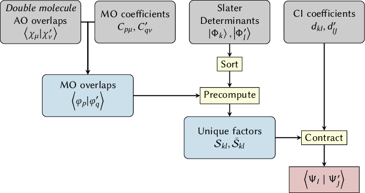
6.35.3 Calling the program
The main program is called in the following form
wfoverlap.x [-m <mem=1000>] [-f <input_file=cioverlap.input>]
with the command line options
- -m : amount of memory in MB
- -f : input file
Example:
wfoverlap.x -m 2000 -f wfov.in
Mode
The program automatically detects whether overlaps or Dyson orbitals should be calculated.
If the number of electrons in the bra and ket wavefunctions is the same, wavefunction overlaps are computed.
If the number of α electrons or the number of β electrons differ by exactly 1, Dyson orbitals are computed.
If the wave functions differ by more than one electron, the program will stop with an error message.
Memory
The amount of memory given is a decisive factor for the performance of the code.
Depending on the amount of memory, one of three different modes is chosen:
(i) All Skl and ―Skl terms are kept in core (using arrays called P_ovland Q_ovl).
(ii) Only the Skl factors (P_ovl) are kept in core. This is indicated by
Allocation of Q block overlap matrix failed.
- Using on-the-fly algorithm for Q determinants.
This mode is generally as efficient as 1. but shows somewhat worse parallel scaling.
(iii) Not even all Skl factors can be stored
Only 437 out of 886 columns of the P_ovl matrix are stored in memory (3 MB)!
Increase the amount of memory to improve the efficiency.
This mode is significantly slower than (i) and (ii) and should be avoided by increasing the amount of memory.
Input file
| Keyword | Default | Description |
| a_mo | – | MO coefficient file (bra) |
| b_mo | – | MO coefficient file (ket) |
| a_mo_read | 0 | Format for the MO coefficients (bra): |
| 0: COLUMBUS, 1: MOLCAS, 2: TURBOMOLE | ||
| b_mo_read | 0 | Format for the MO coefficients (ket) |
| a_det | – | Determinant file (bra) |
| b_det | – | Determinant file (ket) |
| ncore | 0 | Number of discarded core orbitals |
| ndocc | 0 | Number of doubly occupied orbitals that are not used for annihilation in Dyson orbital calculations (only has effect if larger than ncore) |
| ao_read | 0 | Format for overlap integrals: |
| 0: ASCII, 1: MOLCAS, 2: COLUMBUS/SIFS, | ||
| -1: Compute by inversion of MO coefficient matrx | ||
| mix_aoovl | S_mix/ONEINT/aoints | AO overlap file |
| for ao_read=0/1/2 | ||
| same_aos | .false. | If both calculations were performed with the same set of AOs (specify only for ao_read=1/2) |
| nao_a | automatic | Number of bra AOs for ao_read=1/2 (specify only if different from ket AOs) |
| nao_b | automatic | Number of ket AOs (see above) |
| moprint | 0 | Print Dyson orbitals: 1: coefficients to std. out, |
| 2: as Jmol script | ||
| force_direct_dets | .false. | Compute Skl terms directly (turn off ßuperblocks”). Recommended if the number of CPU-cores is large (on the same order as the number of ßuperblocks”). |
| force_noprecalc | .false. | Do not precalculate the ―Skl factors. |
| mixing_angles | .false. | Compute mixing angles as a matrix logarithm. |
An example input file is shown below:
a_mo=mocoef_a
b_mo=mocoef_b
a_det=dets_a
b_det=dets_b
ao_read=2
same_aos
The full list of keywords is given in Table 6.50.
6.35.4 Input data
Typically, three types of input need to be provided: AO overlaps, MO coefficients, and a combined file with determinant information and CI coefficients (cf. Figure 6.5).
The file formats are explained here.
Within SHARC, these files are automatically extracted or converted by the interfaces, so the user does not need to create them.
AO overlaps
The mixed AO overlaps < χμ|χν′ > between the AOs used to expand the bra and ket wavefunctions are required.
They are in general created by a “double molecule” calculation, i.e. an AO integral calculation where every atom is found twice in the input file.
The native format (ao_read=0) is a simple ASCII file containing the relevant off-diagonal block of the mixed AO overlap matrix, e.g.
   7 7
     9.97108464676133E-001    2.36720699813181E-001   ...
     2.36720699813181E-001    9.99919192433940E-001   ...
     1.00147985713321E-002    6.52340422397770E-003   ...
         ...
In addition, MOLCAS (ao_read=1) and COLUMBUS/SIFS (ao_read=2) files can be read in binary form.
If the same AOs are used for the bra and ket wavefunctions and the MO coefficient matrix is square, it is possible to reconstruct the overlaps by inversion of the MO coefficient matrix (ao_read=-1).
In this case it is not necessary to supply a mix_aoovl file.
MO coefficients
MO coefficients of the bra and ket wavefunctions can usually be read in directly in the form written by the quantum chemistry program.
The supported options for a_mo_read and b_mo_read are 0 for COLUMBUS format, 1 for MOLCAS lumorb format, and 2 for TURBOMOLE format.
Because the number of electrons strongly affects the run time of wfoverlap.x, it is generally beneficial to apply a frozen core approximation, even if the actual wave function calculation did not do so.
Most interfaces which use wfoverlap.x have a keyword numfrozcore in the resource file, which only affects the number of frozen core orbitals for the overlap calculation (If the interface support frozen core for the quantum chemistry itself, there will be a keyword in the template file).
Slater determinants and CI coefficients
Slater determinants and CI coefficients are currently supplied by an ASCII file of the form
3 7 168
dddddee   0.979083342437    0.979083342437   -0.122637656388
ddddabe  -0.094807515471   -0.094807515471   -0.663224542162
ddddbae   0.094807515471    0.094807515471    0.663224542162
...
The first line specifies
- the number of states (columns in the file),
- the number of MOs (length of the determinant strings), and
- the number of determinants in the file (length of the file).
Every subsequent line gives the determinant string and the corresponding CI coefficients for the different states.
The following symbols are used in the determinant string:
-
d – doubly occupied
a – singly occupied (α)
b – singly occupied (β)
e – empty
Most relevant for SHARC users, the wfoverlap.x program fully considers all determinants inside these files, without applying any form of truncation. Hence, truncation of long wave functions is done during the creation of the determinant files.
Most interfaces which write these files have a keyword wfthres in their resource file. This threshold is a number between 0.0 and 1.0, and is the minimum wave function norm to which the wave functions should be truncated. During truncation, the interfaces generally retain the largest-amplitude CI coefficients, and remove determinants with small coefficients, i.e., they find the truncated expansion with the fewest determinants which has a norm above the wfthres.
Choosing this threshold properly can very strongly affect the computational time spent in the overlap calculation. Generally, for CASSCF wave functions the threshold can be set to 1 (SHARC_MOLPRO.py, SHARC_MOLCAS.py, and SHARC_BAGEL.py always use all determinants and do not have the wfthres option), for TDA-DFT/ADC(2) it should usually be well above 0.99, for and for MRCI wave functions it might be necessary to go as low as 0.95, depending on the accuracy and performance needed.
For TD-DFT calculations without the Tamm-Damcoff approximation, the response vectors are usually normalized to |X|2−|Y|=1, but only X is used in the overlap calculation; since the norm of X can thus exceed 1, the wfthres should be increased above 1, too.
As a rule of thumb, the threshold should always be chosen such that each state is represented by at least a few 100 determinants in the file, in order to obtain smoothly varying overlaps.
If unsure, the user should perform a test calculation, varying the wfthres until a suitable one is found (i.e., with as many determinants as possible such that the cost of the overlap calculation is bearable).
6.35.5 Output
Usually, the output of wfoverlap.x is automatically extracted by the interfaces, and reported in QM.out in the overlap or 2D-property sections.
Wavefunction overlaps
The output first lists some information about the wavefunction structure and about the computational time taken for the individual steps (cf. Figure 6.5).
A typical result of a wavefunction overlap computation is shown here:
 Overlap matrix <PsiA_i|PsiB_j>
                |PsiB  1>     |PsiB  2>
<PsiA  1|    0.5162656622 -0.2040109070
<PsiA  2|   -0.2167057391 -0.5266552021
 Renormalized overlap matrix <PsiA_i|PsiB_j>
                |PsiB  1>     |PsiB  2>
<PsiA  1|    0.5162656622 -0.2040109070
<PsiA  2|   -0.2167057391 -0.5266552021
 Performing Lowdin orthonormalization by SVD...
 Orthonormalized overlap matrix <PsiA_i|PsiB_j>
                |PsiB  1>     |PsiB  2>
<PsiA  1|    0.9273847015 -0.3741090956
<PsiA  2|   -0.3741090956 -0.9273847015
Overlap matrix gives the raw overlap values

|
(6.25) |
of the wavefunctions supplied.
Renormalized overlap matrix gives the renormalized overlap values
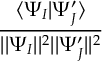
|
(6.26) |
relevant in the case of wavefunction truncation.
The Orthonormalized overlap matrix is constructed according to a procedure described in more detail in Ref. [58].
Dyson orbitals
The matrix of Dyson norms is printed at the end of the file
 ALPHA ionization
 Dyson norm matrix |<PsiA_i|PsiB_j>|^2
                |PsiB  1>     |PsiB  2>     |PsiB  3>
<PsiA  1|    0.8817323437  0.4716319904  0.0680618001
<PsiA  2|    0.0615587916  0.4657174978  0.8772909828
<PsiA  3|    0.0000000000  0.0363130811  0.0000000000
<PsiA  4|    0.9634885049  0.0000000000  0.0017379586
<PsiA  5|    0.0000000000  0.9261839484  0.0000000000
In the case of moprint=1 the orbitals are printed, as well.
The expansion is given with respect to the MOs of the neutral system.
  Dyson orbitals in reference |ket> MO basis:
<PsiA  1|
         |PsiB   1>      |PsiB   2>      |PsiB   3>
MO     1 -1.24032037E-03  0.00000000E+00  9.98160731E-04
MO     2 -5.90277699E-02  0.00000000E+00  6.14517859E-02
MO     3 -1.23295110E-09  0.00000000E+00  3.08416849E-10
MO     4  0.00000000E+00 -6.86713110E-01  0.00000000E+00
MO     5  9.31351013E-01  0.00000000E+00 -2.49427166E-01
MO     6 -3.50106110E-02  0.00000000E+00  4.19935829E-02
MO     7 -1.83303166E-10  0.00000000E+00 -3.67409953E-12
MO     8 -1.91183349E-10  0.00000000E+00  9.40768334E-11
...
Chapter 7 Auxilliary Scripts
In this chapter, all auxiliary scripts and programs are documented. Input generators (like molpro_input.py and molcas_input.py) are documented in the relevant interface sections.
All auxiliary scripts are either interactive-prompting user input from stdin in order to setup a certain task-or non-interactive, meaning they are controlled by command-line arguments and options, in the same way as many standard command-line tools work.
All interactive scripts sequentially ask a number of questions to the user. In many cases, a default value is presented, which is either preset or detected by the scripts based on the availability of certain files. Furthermore, the scripts feature auto-completion of paths and filenames (use TAB), which is active only in questions where auto-completion is relevant. For certain questions where lists of integers needs to be entered, ranges can be indicated with the tilde symbol (), e.g., -8-2 (note that no spaces are allowed between the tilde and the two numbers) to indicate the list -8 -7 -6 -5 -4 -3 -2.
All interactive scripts write a file called KEYSTROKES.<script_name> which contains the user input from the last completed session. These files can be piped to the interactive scripts to perform the same task again, for example:
user@host> cat KEYSTROKES.excite - | $SHARC/excite.py
Note the -, which tells cat to switch to stdin after the file ends, so that the user can proceed if the script asks for more input than contained in the KEYSTROKES file.
All non-interactive scripts can be called with the -h option to obtain a short description, usage information and a list of the command line options.
Non-interactive scripts also write a KEYSTROKES.<script_name> file, which will contain the last command entered to execute the script (including all options and arguments).
All scripts can be safely killed during a run by using Ctrl-C. In the case of interactive scripts, a KEYSTROKES.tmp file remains, containing the user input made so far. Note that the KEYSTROKES.tmp file cannot be directly piped to the scripts, because KEYSTROKES.tmp will be overwritten when the script starts.
7.1 Wigner Distribution Sampling: wigner.py
The first step in preparing the dynamics calculation is to obtain a set of physically reasonable initial conditions. Each initial condition is a set of initial atomic coordinates, initial atomic velocities and initial electronic state. The initial geometry and velocities can be obtained in different ways. With SHARC, often sampling of a quantum-harmonic Wigner distribution is performed.
The sampling is carried out with the non-interactive Python script wigner.py. The theoretical background is summarized in Section 8.24.
7.1.1 Usage
The general usage is
user@host> $SHARC/wigner.py [options] filename.molden
wigner.py takes exactly one command-line argument (the input file with the frequencies and normal modes), plus some options. Usually, the -n option is necessary, since the default is to only create 3 initial conditions.
The argument is the filename of the file containing the information about the vibrational frequencies and normal modes. The file is by default assumed to be in the MOLDEN format. For usage with wigner.py, only the following blocks have to be present:
|
The script accepts a number of command-line options, specified in table 7.1.
| Option | Description | Default |
| -h | Display help message and quit | – |
| -n INTEGER | Number of initial conditions to generate | 3 |
| -m | Modify atom masses (starts interactive dialog) | Most common isotopes |
| -s FLOAT | Scaling factor for the frequencies | 1.0 |
| -t FLOAT | Use Boltzmann-weighted distribution at the given temperature | 0.0 K |
| -T | Discard very high vibrational states at high temperatures | Don’t discard, but warn |
| -L FLOAT | Discard frequencies below the given one (in cm−1) | 10.0 |
| -o FILENAME | Output filename | initconds |
| -x | Creates an xyz file with the sampled geometries | initconds.xyz |
| -l | Instead of generating initconds, create input for SHARC_LVC.py | Create initconds |
| -r INTEGER | Seed for random number generator | 16661 |
| -f F | Type of normal modes read (0=detect automatically, 1-4=see below) | 0 |
| -keep_trans_rot | Do not remove translations and rotations from velocity vector | Remove them |
| -use_eq_geom | Sample only velocities, but keep equilibrium geometry | Sample normally |
| -use_zero_veloc | Sample only geometries, but set velocities to zero | Sample normally |
| -dummy_molecule | Produce a file with n initial conditions for a single hydrogen atom at the origin and zero velocities | |
| -single_atom EL | Produce a file with n initial conditions for a single atom of element EL at the origin and zero velocities | |
| -VASP_masses | Use atomic mass values as defined in VASP. Should be activated if frequencies (phonons) were computed with the VASP code. | Disabled |
7.1.2 Normal mode types
The normal mode vectors contained in a MOLDEN file can follow different conventions, e.g., unscaled Cartesian displacements or different kinds of mass-weighted displacements.
By default, wigner.py attempts to identify which convention is followed by the file (by performing different renormalizations and checking if the so-obtained matrix is orthogonal).
In order to use this automatic detection, use -f 0, which is the default.
Otherwise, there are four possible options: -f 1 to assume normal modes in the GAUSSIAN convention (used by GAUSSIAN, TURBOMOLE, Q-CHEM, ADF, and ORCA); -f 2 to assume Cartesian normal modes (used by MOLCAS and MOLPRO); -f 3 to assume the COLUMBUS convention; or -f 4 for mass-weighted, orthogonal normal modes.
7.1.3 Non-default masses
When the -m option is used, the script will ask the user to interactively modify the atom masses. For each atom (referred to by the atom index as in the MOLDEN file), a mass can be given (relative atomic weights). Note that the frequency calculation which produces the MOLDEN should be done with the same atomic masses.
7.1.4 Sampling at finite temperatures
When the -t option is used, the script assumes a finite, non-zero temperature.
The sampling will then consist of two steps, where first randomly a vibrational state is picked from the Boltzmann distribution, and then the Wigner distribution of that state is employed.
For more details, see Section 8.24.
At high temperatures and for low-frequency modes it is possible that very large vibrational quantum numbers will be selected.
Because of the occurrence of factorials in the Laguerre polynomials in the excited Wigner distributions, this leads to variable overflow for νvib > 150. Hence, the highest vibrational quantum number considered is 150, and higher ones are set to 150.
Since this can lead to an overrepresentation of νvib=150, with the -T option one can instead discard all samplings where νvib > 150.
No matter whether -T is used or not, keep in mind that usually such high vibrational states might invalidate the assumption of an harmonic oscillator, and other sampling methods (e.g., molecular dynamics) should be considered.
7.1.5 Output
The script wigner.py generates a single output file, by default called initconds. All information about the initial conditions is stored in this file. Later steps in the preparation of the initial conditions add information about the excited states to this file. The file is formatted in a human-readable form.
The initconds file format is specified in section 7.10.4.
When the -x option is given, additionally the script produces a file called initconds.xyz, which contains the sampled geometries in standard xyz format. This can be useful to inspect the distribution of geometry parameters (e.g., bond lengths) or to perform single point calculations at the sampled geometries.
When the -l option is given, the script only produces a file called V0.txt, which is a necessary input file for the LVC interface (see section 6.4). If this option is activated, no initconds or initconds.xyz files are produced.
7.2 Vibrational State Selected Sampling: wigner_state_selected.py
In addition to wigner.py one can use wigner_state_selected.py to perform vibrational-state-selected initial conditions.
In that situation, one can specify the vibrational level for each normal mode.
7.2.1 Usage
The general usage is
user@host> $SHARC/wigner_state_selected.py [options] filename.molden
wigner_state_selected.py takes exactly one command-line argument (the input file with the frequencies and normal modes), plus some options. Usually, the -vibselec, -vibdist, -vibstate or -vibene, and -n options are necessary, the default is to only create 3 initial conditions.
Like wigner.py, the argument is the filename of the file containing the information about the vibrational frequencies and normal modes. The file is by default assumed to be in the MOLDEN format.
Only the following blocks have to be present:
- [FREQ]
- [FR-COORD]
- [FR-NORM-COORD]
The script accepts a number of command-line options, specified in Table 7.2.
The descriptions of the main options -vibselect, -vibdist, -vibstate, -vibene, -method, and -template will be described in next section.
| Option | Description | Default |
| -vibselect | Method for the vibrational energy (possible: 1, 2, 4-7). | 6 |
| -vibdist | Method for the phase space distribution (possible: 0, 1, 2). | 0 |
| -vibstate | List of vibrational state for each mode. | 0 |
| -viblist | Method to assign mode with the non-zero vibrational level. | 0 |
| -vibene | List of vibrational energy for each model | 0.0 |
| -method | Method for the computation of the energy (possible: 0, 1) | 0 |
| -template | name of the template file to interface with electronic structure (see below). This is only needed when using -method 1. | |
| -h | Display help message and quit | – |
| -n INTEGER | Number of initial conditions to generate | 3 |
| -m | Modify atom masses (starts interactive dialog) | Most common isotopes |
| -s FLOAT | Scaling factor for the frequencies | 1.0 |
| -t FLOAT | Use Boltzmann-weighted distribution at the given temperature | 0.0 K |
| -T | Discard very high vibrational states at high temperatures | Don’t discard, but warn |
| -L FLOAT | Discard frequencies below the given one (in cm−1) | 10.0 |
| -o FILENAME | Output filename | initconds |
| -x | Creates an xyz file with the sampled geometries | initconds.xyz |
| -r INTEGER | Seed for random number generator | 16661 |
| -f F | Type of normal modes read (0=detect automatically, 1-4=see below) | 0 |
| -keep_trans_rot | Do not remove translations and rotations from velocity vector | |
| -use_eq_geom | Sample only velocities, but keep equilibrium geometry | Sample normally |
| -use_zero_veloc | Sample only geometries, but set velocities to zero | Sample normally |
7.2.2 Major options
The wigner_state_selected.py script involves five major options to perform vibrational state selection.
-vibselect determines the method to select the vibrational mode energy:
-
-vibselect 1: the user will provide a list of vibrational quantum numbers; this will require the keyword -vibstate.
-vibselect 2: the program will assign vibrational quantum numbers for each mode. This assignment is random, and selected out of a Boltzmann distribution at a user-specified temperature from option -t.
-vibselect 3: the program generates an initial velocity from a Maxwell thermal distribution at a given temperature from option -t. This is an option for canonical ensembles, not an option for state-selected ensembles. This option is not available at the moment.
-vibselect 4: the amount of energy in each mode is the same, and is set by option -vibene E, where E is the energy of each mode in eV.
-vibselect 5: the amount of energy in each mode is different, and is set option by -vibene E1,E2,E3,..., where E1,E2,E3,... is a list of energies in eV for each mode.
-vibselect 6: default, similar as -vibselect 4, but the energy of each mode is computed as minimum of zero point energy and E.
-vibselect 7: similar as -vibselect 5, but the energy of each mode is computed as minimum of zero point energy and EI, where I is the index of the mode.
-vibdist determines the type of phase space distribution:
-
-vibdist 0: default, uses quasiclassical or classical distribution. It is a uniform distribution. It is quasiclassical if vibselect=1 or 2 and classical if vibselect ≥ 4.
-vibdist 1: ground state harmonic oscillator distribution.
-vibdist 2: Wigner distribution.
-vibstate is a quantum number for all modes or list of vibrational quantum numbers for each mode.
For example, -vibstate 0 specifies all vibrational mode with quantum number 0, i.e. all mode have only zero point energy.
-vibstate 0,1,2,... specifies the quantum number for each mode, in this example, the first three modes have vibrational quantum numbers 0, 1, and 2, respectively.
-viblist is a list of vibrational quantum numbers for all modes whose vibrational quantum number are non-zero, and the rest modes are all set to zero.
This is convenient if one is setting up an initial condition for which most modes’ vibrational quantum number are zero, and only several modes’ quantum number are non-zero. For example, -viblist 1,1?5,3 specifies all vibrational mode with 0 quantum number, except mode 1 and mode 5; mode 1 has vibrational quantum number 1, and mode 5 has vibrational quantum number 3.
Pairs of numbers, i.e., mode and corresponding vibrational quantum number are separated by “?”.
-vibene is a vibrational energy for all modes or a list of vibrational energies for each mode.
For example, -vibene 0.2 specifies all vibrational mode with 0.2 eV of vibrational energy.
-vibene 0.1,0.2,0.1,... specifies the vibrational energy for each mode, in this example, the first three modes have vibrational energies of 0.1 eV, 0.2 eV, and 0.1 eV, respectively.
-method determines how energies are computed for geometries away from the equilibrium structure.
With the default -method 0, the harmonic oscillator approximation, using the provided normal modes, is used.
With -method 1, at each geometry an electronic structure calculation is performed, using the additional option -template, which specifies a script that interfacing with electronic structure calculations.
Note that -method 1 is not recommended, because one can also perform electronic structure calculations at all displaced geometries later, using setup_init.py and the SHARC interfaces.
This allows to use all interfaced methods out-of-the-box without needing to write a template script, and is better supported in the rest of the SHARC workflow.
-template keyword follows by a file name that is a script serves as interface between the wigner_state_selected.py and electronic structure software.
When using ab initio potential, i.e., when set -method 1, the wigner_state_selected.py will write a file called tmp_state_selected.xyz everytime it samples a new geometry, and execute the script, then read the energy from an output file called energy_state_selected.
Therefore, the function of this user-defined script is to read tmp_state_selected.xyz, and write energy into file energy_state_selected.
See the next subsection for an example.
7.2.3 Template
The following bash script shows an example of a template.
The script reads the tmp_state_selected.xyz, write a Gaussian density functional calculation with MN15 functional and def2-TZVP basis set, and stores the density functional energy into file energy_state_selected.
#!/bin/bash
#write a Gaussian input
echo "%Chk=e.chk" > e1.tmp
echo "%Mem=11800mb" >> e1.tmp
echo "#P def2TZVP SCF=(Tight,novracc,maxcycle=500) Integral(Grid=UltraFine) MN15" >> e1.tmp
echo "  " >> e1.tmp
echo "my molecule" >> e1.tmp
echo "0  1" >> t1.tmp
echo "  " > e2.tmp
echo "  " >> e2.tmp
cat e1.tmp tmp_state_selected.xyz e2.tmp > e.com
#run a Gaussian calculation
/software/g09/g09 < e.com > e.out
#save the energy into energy_state_selected
grep 'SCF Done' e.out|awk '{print $5}' > energy_state_selected
7.2.4 Normal mode types
The normal mode vectors contained in a MOLDEN file can follow different conventions, e.g., unscaled Cartesian displacements or different kinds of mass-weighted displacements.
By default, wigner_state_selected.py attempts to identify which convention is followed by the file (by performing different renormalizations and checking if the so-obtained matrix is orthogonal).
In order to use this automatic detection, use -f 0, which is the default.
Otherwise, there are four possible options: -f 1 to assume normal modes in the GAUSSIAN convention (used by GAUSSIAN, TURBOMOLE, Q-CHEM, ADF, and ORCA); -f 2 to assume Cartesian normal modes (used by MOLCAS and MOLPRO); -f 3 to assume the COLUMBUS convention; or -f 4 for mass-weighted, orthogonal normal modes.
7.2.5 Non-default masses
When the -m option is used, the script will ask the user to interactively modify the atom masses. For each atom (referred to by the atom index as in the MOLDEN file), a mass can be given (relative atomic weights). Note that the frequency calculation which produces the MOLDEN should be done with the same atomic masses.
7.2.6 Output
The script wigner_state_selected.py generates a single output file, by default called initconds. All information about the initial conditions is stored in this file. Later steps in the preparation of the initial conditions add information about the excited states to this file. The file is formatted in a human-readable form.
The initconds file format is specified in section 7.10.4.
When the -x option is given, additionally the script produces a file called initconds.xyz, which contains the sampled geometries in standard xyz format. This can be useful to inspect the distribution of geometry parameters (e.g., bond lengths) or to perform single point calculations at the sampled geometries.
7.3 Initial condition for collision dynamics: bimolecular_collision.py
The script bimolecular_collision.py is used in the preparation and sampling of initial conditions for bimolecular collision processes.
This is achieved by merging initconds files from other sources (e.g., wigner.py or wigner_state_selected.py).
There are two operation modes.
If one is performing a molecule + molecule collision dynamics, one needs to provide two initconds files.
For a molecule + atom collision dynamics, one needs to provide only oneinitconds file and additionally the element of the colliding atom.
7.3.1 Usage
To set up an initial condition for colliding two molecules (here we simply call an atom a special case of molecule to simplify the discussion), the following collision parameters are required: initial separation of the two molecules, impact parameter, and collision energy.
Notice that, currently, setting up relative angular momenta between the two molecules is not supported.
The general usage for a molecule + molecule collision process is:
user@host> $SHARC/bimolecular_collision.py [options] initconds1 initconds2
and for a molecule + atom process it is:
user@host> $SHARC/bimolecular_collision.py [options] initconds1
bimolecular_collision.py takes one or two command-line arguments (the initconds files), plus some options.
Usually, the -bmin, -bmax, -separation, -relative_trans, and -n options are necessary.
The default is to only create 1 initial conditions.
The list of all available options are shown in Table 7.3.
| Option | Description | Default |
| -atom | The element used in molecular + atom collision dynamics (string). | “H” |
| -bmin | minimum of impact parameter. | 0.0 (Å) |
| -bmax | maximum of impact parameter. | 5.0 (Å) |
| -strata | number of strata used in sampling impact parameter. | 1 |
| -separation | initial separation between the two molecules | 10.0 (Å) |
| -relative_trans | relative translational energy between the two molecules. | 1.0 (eV) |
| -no_random_orient | not randomly re-orient each molecules. | False |
| -n INTEGER | Number of initial conditions to generate | 3 |
| -o FILENAME | Output filename | initconds |
| -x | Creates an xyz file with the sampled geometries | initconds.xyz |
7.3.2 Usage
The bimolecular_collision.py has seven major options.
-atom to specify the element used in molecule + atom collision dynamics. For example, -atom "H", to specify a hydrogen atom.
Three options are used to randomly sample the impact parameter, where -bmin specifies the minimum impact parameter, -bmax specifies the maximum impact parameter, and -strata specifies how many strata are used in the stratified sampling of impact parameter.
For example, -bmin 0.0 -bmax 5.0 -strata 1 means the sampled impact parameter is in range 0.0 to 5.0 Å.
Instead, -bmin 0.0 -bmax 5.0 -strata 2 means the first half of the initial conditions have impact parameter in range 0.0 to 2.5 Å, and the second half of the initial conditions have impact parameter in range of 2.5 to 5.0 Å.
The stratified sampling is especially useful when trying to analyze the opacity function at the end of the trajectory simulation, i.e., one can observe how cross section changes as a function of impact parameter, and if the simulation is converged with respect to the impact parameter.
-separation sets the initial separation of the center of mass of the two molecules. The default value is 10 Å.
-relative_trans sets the initial relative translational energy between the two molecules in units of eV. The default is 1.0 eV.
Note that we are always letting molecule 2 collide towards molecule 1, so molecule 2 will receive the translational energy.
-no_random_orient prevents the initial random re-orientation of the molecules.
Note that when we put two molecules together, one can re-orient each of the two molecules, and this is done by default.
7.4 AMBER Trajectory Sampling: amber_to_initconds.py
The first step in preparing the dynamics calculation is to obtain a set of physically reasonable initial conditions. Each initial condition is a set of initial atomic coordinates, initial atomic velocities and initial electronic state. The initial geometry and velocities can be obtained in different ways.
Besides sampling from a quantum mechanical Wigner distribution (with wigner.py), it is a widespread approach to sample geometries and velocities from a ground state molecular dynamics simulation.
Using amber_to_initconds.py, one can convert the results of an AMBER simulation to a SHARC initconds file.
Note that one can instead work with restartnc_to_xyz.py (see Section 7.7), which is more complicated to use but avoids huge initconds files in very large projects.
7.4.1 Usage
In order to use amber_to_initconds.py, it is necessary to first carry out an AMBER simulation.
You need to add the following options to the AMBER MD input file: (i) ntxo=1 to tell AMBER to write ASCII restart files, (ii) ntwr=-5000 to create a restart file every 5000 steps (other values are possible, but use the minus to not overwrite the restart files).
This will create a set of AMBER restart files called, e.g., md.rst_5000, md.rst_10000, …
Note that it is also necessary to reimage the AMBER restart files, because SHARC does not work with periodic boundary conditions, but the AMBER trajectories might use them.
The reimaging can be performed with AMBER‘s tool cpptraj, using the following input:
parm <filename>.prmtop
trajin <filename>.rst7
autoimage
trajout <filename2>.rst7
run
This command has to be repeated for each restart file which needs to be reimaged.
Note that amber_to_initconds.py only works with the rst7 ASCII file format, not with the rst format (even if it is ASCII-formatted).
If you saved the restart files in AMBER‘s newer NetCDF format, cpptraj can also be used to convert them to ASCII rst7 restart files.
If you did not save restart files, cpptraj can even be used to generate restart files from the trajectory file (.mdcrd and .mdvel), but for this way it is necessary to save the velocities (.mdvel file).
With the restart files prepared, call amber_to_initconds.py like this:
user@host> $SHARC/amber_to_initconds.py [options] md.prmtop md.rst_0 md.rst_5000 md.rst_10000 ...
The possible options are shown in Table 7.4.
| Option | Description | Default |
| -h | Display help message and quit | – |
| -t FLOAT | Time step (in femtoseconds) used in the AMBER simulation | – |
| -o FILENAME | Output filename | initconds |
| -x | Creates an xyz file with the sampled geometries | initconds.xyz |
| -m | Modify atom masses (starts interactive dialog) | As in prmtop file |
| -keep_trans_rot | Do not remove translations and rotations from velocity vector | |
| -use_zero_veloc | Sample only geometries, but set velocities to zero | Sample normally |
7.4.2 Time Step
Note that the option -t (giving the time step used in AMBER in femtoseconds) is mandatory; if not given, an error message is produced.
This is because AMBER uses a Leapfrog algorithm and thus stores in the restart file R(t) and v(t−∆t/2), whereas SHARC uses the velocity-Verlet algorithm and requires geometry and velocity at the same time, e.g., R(t−∆t/2) and v(t−∆t/2).
To compensate this, amber_to_initconds.py computes R(t−∆t/2) from R(t)−v(t−∆t/2)∆t/2.
Hence, ∆t of the AMBER trajectory needs to be known.
7.4.3 Atom Types and Masses
By default, atom types and masses are read from the prmtop file (from flags ATOMIC_NUMBER and MASS).
If the atomic number is not sensible (e.g., -1 for a transition metal) then amber_to_initconds.py prompts the user to define the element.
The masses in the prmtop file can be overridden if the -m option is given; then the user can adjust the mass of each atom individually.
7.4.4 Output
amber_to_initconds.py produces the same output as wigner.py (section 7.1).
By default, a file called initconds is generated for the converted initial conditions.
It is important to note that the first restart file given (the second command line argument) is treated as the “equilibrium” geometry for the purpose of generating the initconds file.
The second given restart file is then converted to the initial condition with index 1, and so on.
Note that it is possible to give the same restart file multiple times as an argument (so that the same geometry can be used as “equilibrium” geometry and as proper initial condition.
7.5 VASP Trajectory Sampling: vasp_to_initconds.py
The first step in preparing the dynamics calculation is to obtain a set of physically reasonable initial conditions. Each initial condition is a set of initial atomic coordinates, initial atomic velocities and initial electronic state. The initial geometry and velocities can be obtained in different ways.
Besides sampling from a quantum mechanical Wigner distribution (with wigner.py), it is a widespread approach to sample geometries and velocities from a ground state molecular dynamics simulation.
Using vasp_to_initconds.py, one can convert the results of a VASP ground-state ab-initio molecular dynamics (MD) simulation to a SHARC initconds file. This could be particularly useful when using the SHARC– VASP interface (Sec.6.13).
7.5.1 Usage
In order to use vasp_to_initconds.py, it is necessary to first carry out a VASP molecular dynamics simulation. Note that VASP must be compiled with HDF5 support and both py4vasp and mdtraj python packages have to be installed in the user’s conda environment for a complete functioning of vasp_to_initconds.py. Indeed, vasp_to_initconds.py reads the VASP MD data through the .h5 files generated by VASP. Additionally, atomic velocities have to be written out in the .f5 files, which means VELOCITY=.true. has to be set in the INCAR file before the MD run is started. Note that this script considers as default value for atomic masses the VASP default atomic masses, which are usually specified in the POTCAR files. User-modified atomic masses can be provided with the -m flag but they have to be consistently used in the MD run.
Once the results of a VASP MD run are sorted, call vasp_to_initconds.py like this:
user@host> $SHARC/vasp_to_initconds.py path_to_MD_directory path_to_POSCAR_eq [options]
The possible options are shown in Table 7.5.
Note that the second keyword argument “path_to_POSCAR_eq” must be passed as well to specify the path to the POSCAR file containing the equilibrium structure of the system under investigation.
This is to generate a reasonable reference structure for the ICOND_00000 initial condition and align each sampled frame of the MD run to a meaningful reference.
| Option | Description | Default |
| -h | Display help message and quit | – |
| -f INTEGER | Number of last frames of the MD run that will be processed for generating initial conditions | all frames are analyzed |
| -n INTEGER | Number of initial conditions that will be generated | 10 |
| -random | Generate the selected number of initial conditions by random picking among the processed frames. | |
| -every | The whole set of processed frames is divided into consecutive subgroups of (possibly) the same size whose number equal the number of specified initial conditions to be sampled. One frame is taken from each subgroup and the corresponding initial condition is generated. | |
| -o FILENAME | Output filename | initconds |
| -x | Creates an xyz file with the sampled geometries | initconds.xyz |
| -m | Modify atom masses (starts interactive dialog) | Uses default VASP atomic masses |
| -keep_trans_rot | Do not remove translations and rotations from velocity vector |
7.5.2 Output
vasp_to_initconds.py produces the same output as wigner.py (section 7.1).
By default, a file called initconds is generated for the converted initial conditions.
It is important to note that the first frame of the MD trajectory is treated as the “equilibrium” geometry for the purpose of generating the initconds file.
7.6 SHARC Trajectory Sampling: sharctraj_to_initconds.py
The first step in preparing the dynamics calculation is to obtain a set of physically reasonable initial conditions. Each initial condition is a set of initial atomic coordinates, initial atomic velocities and initial electronic state. The initial geometry and velocities can be obtained in different ways.
Besides sampling from a quantum mechanical Wigner distribution, it is often appropriate to sample geometries and velocities from a ground state molecular dynamics simulation.
Using sharctraj_to_initconds.py, one can convert the results of a SHARC simulation to a new SHARC initconds file.
The script has two modes.
In the default mode, the user provides a set of trajectories, as well as a range of time steps to sample from, and the script selects randomly exactly one time step from each given trajectory to extract.
Alternatively, in single trajectory mode (with the -give_single_out and -s options) the scripts extracts snapshots at equal spacing from a single trajectory.
7.6.1 Usage
In order to use sharctraj_to_initconds.py, it is necessary to first run a number of SHARC trajectories (the initial conditions for those need to be obtained with wigner.py or amber_to_initconds.py).
The trajectories can be run with any number of states and in any state, and with any desirable options; only geometries and velocities are converted to the new initconds file.
With the trajectories prepared, call sharctraj_to_initconds.py like this:
user@host> $SHARC/sharctraj_to_initconds.py [options] Singlet_0 ...
Alternatively, with the -give_TRAJ_paths option, one can also do:
user@host> $SHARC/sharctraj_to_initconds.py --give_TRAJ_paths [options] TRAJ_00001 TRAJ_00002 ...
The possible options are shown in Table 7.6.
| Option | Description | Default |
| -h | Display help message and quit | – |
| -r INTEGER | Seed for the random number generator | 16661 |
| -S INTEGER INTEGER | Range of time steps from which a step is randomly chosen (with -give_single_out, defines the range from which to sample) | last step (-S -1 -1) |
| -o FILENAME | Output filename | initconds |
| -x | Creates an xyz file with the sampled geometries | initconds.xyz |
| -keep_trans_rot | Do not remove translations and rotations from velocity | Removes translations/rotations. |
| -use_zero_veloc | Sample only geometries, but set velocities to zero | Sample normally |
| -debug | Show timings | |
| -give_TRAJ_paths | Allows specifying individual trajectories | Specify parent directories |
| -give_single_out | Allows specifying a single output.dat file to extract multiple snapshots (select stride with -s, which is required with this option). | Select one random snapshot from each given trajectory. |
| -s INTEGER | Stride for sampling geometries when using -give_single_out (every N-th step is taken) | Required if -give_single_out |
7.6.2 Random Picking of Time Step
In default mode, for each directory specified as command line argument, sharctraj_to_initconds.py picks exactly one time step and extracts geometries and velocities of that time step.
Note that a directory can be given several times as argument, so that multiple time steps can be selected.
The time steps are generally picked randomly (uniform probabilities) from an interval specified with the -S option.
This option takes two integers, e.g., -S 50 -50, which can be positive or negative.
The meaning of positive/negative/zero is the same as in PYTHON: positive numbers simply denote a time step (start counting with zero for the step zero of the trajectory); for negative numbers, start counting at the end, i.e., -1 is the last time step of the trajectory.
In this way, it is possible to select the snapshot from the last n steps of all trajectories, even if they have different length.
The example above, -S 50 -50, means picking a time step between the 50th and the 50th-last step. Note that if a trajectory is shorter than 100 steps, in this example it is skipped because there are no steps between the 50th and the 50th-last step.
7.6.3 Output
sharctraj_to_initconds.py produces the same output as wigner.py (section 7.1).
By default, a file called initconds is generated for the converted initial conditions.
It is important to note that the first directory given (the first command line argument) is treated as the “equilibrium” geometry for the purpose of generating the initconds file.
The second given directory is then converted to the initial condition with index 1, and so on.
Note that it is possible to give the same directory multiple times as an argument (so that the same geometry can be used as “equilibrium” geometry and as proper initial condition.
7.7 Creating an XYZ file from an Amber restart file: restartnc_to_xyz.py
With the script restartnc_to_xyz.py one can extract information from an Amber restart file and write the Cartesian coordinates to different files.
There are three different modes in which the script can operate.
In the default mode, the script is producing output in xyz format.
The velocities from the restart file are discarded.
Optionally, the script can pick up lines from a QM.in file and append to the xyz output.
In the second mode, the script produces output in initconds file format.
In the third mode, the script produces a geom and a veloc file (overwriting previous files in the present folder).
In both cases, the velocities from the restart file are considered.
Note that this script, like amber_to_initconds.py (Section 7.4) modifies the geometries read from the restart file by rewinding half a time step.
This is because Amber uses a Leapfrog algorithm, but SHARC uses the velocity Verlet algorithm.
This is the reason why the time step is a required argument for restartnc_to_xyz.py.
Optionally, the script can also reorder the coordinates of identical residues according to the distance of the residue from a user-defined list of atoms.
In this way, e.g., one could prepare the initial coordinates for SHARC such that the closest waters always come first.
This is useful, e.g., to define a bias potential on a number of outmost water molecules.
For this, the script identifies identical residues from the prmtop file and reorders them automatically.
7.7.1 Usage
restartnc_to_xyz.py is a command line tool, and is executed like this:
user@host> $SHARC/restartnc_to_xyz.py -t <time step> <prmtop file> <restartnc file> > <output file>
The options are summarized in Table 7.7
| Option | Description | Default |
| -h | Display help message and quit. | – |
| -t | Specify the timestep in fs that Amber used | required. |
| -a | Output in Angstrom | in Bohr |
| -q | Append request lines from file ‘QMin’ | do not append anything |
| -i | Produce output to append to initconds | produce output in xyz format |
| -g | Produce geom and veloc files | produce output in xyz format |
| -r | Followed by a string (e.g., "1,3,612") defining the atoms from whose center of mass the atoms should be reordered. | Do not reorder |
| -m | Rather than using COM-COM distances for reordering, use minimum distances. |
7.7.2 Input
Time step
Here, the user needs to specify the timestep that was used for the Amber dynamics (e.g., 2 fs).
The output coordinates will be →Routput=→Rfrom rst − [1/2]∆t →vfrom rst.
Prmtop file
Specify the prmtop file of the system that was propagated in Amber so that the information on atom types etc. can be extracted.
Restartnc file
Specify the Amber restart file (NetCDF format) containing the molecular dynamics data that should be extracted.
7.7.3 Output
The extracted Cartesian coordinates and/or velocities of each time step are put to the terminal in the specified format (XYZ or initconds).
In case of the -g option, the geom and veloc files are written to the current directory.
7.8 Creating an XYZ file from a SHARC trajectory: sharctraj_to_xyz.py
The script sharctraj_to_xyz.py allows extraction of the geometries and velocities of a single time step from a SHARC NetCDF trajectory file and prints or writes them in the same three formats as restartnc_to_xyz.py (XYZ files, QM.in files, and geom/veloc file pairs).
The main application for this script is in reusing geometries and velocities from a finished SHARC trajectory to create new initial conditions.
It shares this task with sharctraj_to_initconds.py, which is intended for smaller projects and ASCII output.dat files and operates on an entire swarm of trajectories to produce a new initconds file.
In contrast, sharctraj_to_xyz.py operates on a single NetCDF output.dat.nc/output_NUC.dat.nc file and is intended for projects where dummy initconds files are used.
7.8.1 Usage
sharctraj_to_xyz.py is a command-line tool and is executed as follows:
user@host> $SHARC/sharctraj_to_xyz.py [options] <geom> <output.dat.nc>
The available command-line options are summarized in Table 7.8.
| Option | Description | Default |
| -h | Display help message and quit. | – |
| -s | Select time step (negative numbers count from the end) | last frame |
| -a | Output in Angstrom | in Bohr |
| -q | Append request lines from file QM.in in same directory | do not append anything |
| -i | Produce output to append to initconds format | print XYZ format |
| -g | Write geom and veloc files | print XYZ format |
Note that in -i and -g modes, the flags -a and -q are ignored.
7.8.2 Input
Geometry file
The geometry file must be in SHARC format, containing atomic symbols, numbers, and masses. It is used to map the structure from the NetCDF file.
NetCDF trajectory file
The trajectory file must be in SHARC NetCDF format and must contain geometry and velocity information. This file is accessed at the selected time step to retrieve the data.
Time step
The desired time step to extract can be specified via the -s flag. Negative numbers count from the last frame backward (e.g., -1 extracts the final step).
Unlike sharctraj_to_initconds.py, sharctraj_to_xyz.py does not have any options to pick a random time step, but because sharctraj_to_xyz.py operates only on a single file, randomization logic can be implemented in a Bash wrapper script.
7.8.3 Output
Three different output modes are available:
- By default, the script prints atomic positions in XYZ format to standard output. Using the -q option, requests from a QM.in file in the same directory can be appended.
- Using the -i option, the output is printed in initconds file format.
- Using the -g option, two files geom and veloc are written to the current directory (overwriting any existing files).
7.9 Setup of Initial Calculations: setup_init.py
The interactive script setup_init.py creates input for single point calculations at the initial geometries given in an initconds file. These calculations might be necessary for some schemes to select the initial electronic state of the trajectory, e.g., based on the excitation energies and oscillator strength of the transitions from ground state to the excited state, or based on overlaps with a reference wave function.
There are other choices of the initial state possible, which do not require single point calculations at all initial geometries. See the description of excite.py (section 7.10). In this case, setup_init.py can be used to set up only the calculation at the equilibrium geometry (see below at “Range of Initial Conditions”).
7.9.1 Usage
The script is interactive, and can be started by simply typing
user@host> $SHARC/setup_init.py
Please be aware that the script will setup the calculations in the directory where it was started, so the user should cd to the desired directory before executing the script.
Please note that the script does not expand or shell variables, except where noted otherwise.
7.9.2 Input
The script will prompt the user for the input. In the following, all input parameters are documented:
Initial Conditions File
Enter the filename of the initial conditions file, which was generated beforehand with wigner.py. If the script finds a file called initconds, the user is asked whether to use this file, otherwise the user has to enter an appropriate filename. The script detects the number of initial conditions and number of atoms automatically from the initial conditions file.
Range of Initial Conditions
The initial conditions in initconds are indexed, starting with the index 1. In order to prepare ab initio calculations for a subset of all initial conditions, enter a range of indices, e.g. a and b. This will prepare all initial conditions with indices in the interval [a,b]. In any case, the script will additionally prepare a calculation for the equilibrium geometry (except if a finished calculation for the equilibrium geometry was found).
If the interval [0,0] is given, the script will only setup the calculation at the equilibrium geometry.
Number of states
Here the user can specify the number of excited states to be calculated. Note that the ground state has to be counted as well, e.g., if 4 singlet states are specified, the calculation will involve the S0, S1, S2 and S3. Also states of higher multiplicity can be given, e.g. triplet or quintet states.
For even-electron molecules, including odd-electron states (e.g. doublets) is only useful if transition properties for ionization can be computed (e.g. Dyson norms with some of the interfaces). These transition properties can be used to calculate ionization spectra or to obtain initial conditions for dynamics after ionization.
Charge per multiplicity
In SHARC4, the molecular charge is not set in the interface template files, but directly by the setup scripts/ SHARC driver/parent interface.
Hence, enter the molecular charge per multiplicity here.
This array needs to have the same length as the number of states array.
If the number of states for some multiplicities is zero, the entered number will be ignored.
For example, if you provided states 3 2 1 and charges 0 +1 0, then the 3 singlets and 1 triplet states will be computed as neutral species, and the 2 doublet states as cations with charge +1.
Interface
In this point, choose any of the displayed interfaces to carry out the ab initio calculations.
Enter the corresponding number.
If you selected SHARC_LEGACY.py, then you have to subsequently select the legacy interface that you intend to use.
If you selected a hybrid interface, then you will subsequently be queried with the path to the corresponding template file, so that the hybrid interface can figure out the child interface it should use.
This might continue recursively until all interfaces in the interface call tree are known.
Spin-orbit calculation
Usually, it is sufficient to calculate the spin-free excitation energies and oscillator strengths in order to decide for the initial state.
However, using this option, the effects of spin-orbit coupling on the excitation energies and oscillator strengths can be included.
Note that the script will not ask for spin-orbit couplings if only singlet states are included in the calculation, or if the chosen interface does not support calculation of spin-orbit couplings.
Dyson norm calculation
In some cases, initial conditions should be set up to simulate dynamics after ionization.
Note that the script will only ask for this property if the chosen interface supports Dyson norms.
Reference overlaps
The calculations can be setup in such a way that the wave function overlaps between states at the equilibrium geometry and the displaced geometries is computed.
This allows correlating the states at the displaced geometries with the reference states, such that one can know the state characters of all states without inspection.
This is useful for a crude “diabatization” of the states, e.g., if one wants to start all trajectories in the nπ* state of the molecule although this state can be S1, S2, or S3 (use excite.py to setup initial conditions in such a way, see section 7.10).
Note that the script will only ask for this option if the chosen interface supports wave function overlaps.
When activating this option, keep in mind that the calculation in ICOND_00000 must be successfully finished before any of the other ICOND_XXXXX calculations can be started.
TheoDORE analysis
If the chosen interface supports wave function analysis with TheoDORE, then this option can be activated here.
setup_init.py will then include the relevant keywords in the computations, and the results of the TheoDORE analysis will be written to the QM.out files.
Note that the script will only ask for this option if the chosen interface supports wave function descriptors from TheoDORE.
The remaining settings for TheoDORE (fragment and descriptor input) will be asked later in setup_init.py.
7.9.3 Interface-specific input
After identifying all electronic structure information that needs to be computed, the setup script will call the chosen interface’s own setup routines.
The interface will ask the user for all necessary information, depending on the requested quantities.
For hybrid interfaces, the children’s setup routines will also be called at some point, possibly in a recursive fashion, until all interfaces in the call tree are setup.
See Chapter 6 for the questions that the interfaces ask.
7.9.4 Input for Run Scripts
Run script mode
The script setup_init.py generates a run script (Bash) for each initial condition calculation. Due to the large variety of cluster architectures, these run scripts might not work in every case. It is the user’s responsibility to adapt the generated run scripts to his needs.
setup_init.py can generate run scripts for two different schemes how to execute the calculations. With the first scheme, the ab initio calculations are performed in the directory where they were setup (subdirectories of the directory where setup_init.py was started). Note that the interfaces will still use their scratch directories to perform the actual quantum chemistry calculations. Currently, this is the default and simplest option.
With the second option, the run scripts will transfer the input files for each ab initio calculation to a temporary directory, where the interface is started. After the interface finishes all calculations, the results files are transferred back to the primary directory and the temporary directory is deleted. Note that setup_init.py in any case creates the directory structure in the directory where it was started. The name of the temporary directory can contain shell variables, which will be expanded when the script is running (on the compute host).
Submission script
The setup script can also create a Bash script for the submission of all ab initio calculations to a queueing system. The user has to provide a submission command for that, including any options which might be necessary. This submission script might not work with all queueing systems.
The user should also enter a project name that is used to add a name option to the submission script.
7.9.5 Output
setup_init.py will create for each initial condition in the given range a directory whose names follow the format ICOND_%05i/, where %05i is the index of the initial condition padded with zeroes to 5 digits. Additionally, the directory ICOND_00000/ is created for the calculation of the excitation energies at the equilibrium geometry.
To each directory, the following files will be added:
- QM.in: Main input file for the interface, contains the geometry and the control keywords (to specify which quantities need to be calculated).
- run.sh: Run script, which can be started interactively in order to perform the ab initio calculation in this directory. Can also be adapted to a batch script for submission to a queue
- Interface-specific files: Usually a template file, a resource file, and an initial wave function.
The calculations in each directory can be simply executed by starting run.sh in each directory. In order to perform this task consecutively on a single machine, the script all_run.sh can be executed. The file DONE contains the progress of this calculation.
Alternatively, each run script can be sent to a queueing system (you might need to adapt this script to you cluster system).
Note that if reference overlaps were requested, the calculation in ICOND_00000/ must be finished before starting any of the other calculations.
In figure 7.1, the directory tree structure setup by setup_init.py is given.
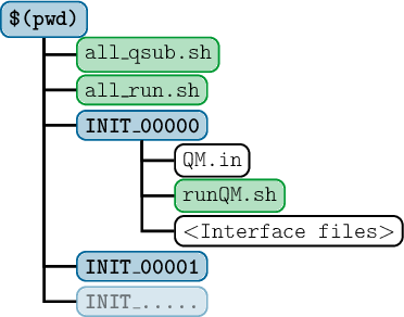
After all calculations are finished, excite.py can be used to collect the results.
7.10 Excitation Selection: excite.py
excite.py has two tasks: adding excited-state information to the initconds file, and deciding which excited state for which initial condition is a valid initial state for the dynamics.
7.10.1 Usage
The script is interactive, and can be started by simply typing
user@host> $SHARC/excite.py
7.10.2 Input
Initial condition file
Enter the path to the initial conditions file, to which excite.py will add excited-state information. This file can already contain excited-state information (in this case this information can be reused).
Generate excited state list
There are three possibilities to add excited-state information to the initconds file:
- generate a list of dummy excited states,
- read excited-state information from the output of the initial ab initio calculations (prepare the calculations with setup_init.py),
- keep the existing excited-state information in the initconds file.
The first option is mainly used if no initial ab initio calculations need to be performed (e.g., the initial state is known).
In order to use the second option, one should first setup initial excited-state calculations using setup_init.py (see 7.9) and run the calculations. excite.py can then read the output of the initial calculations and calculate excitation energies and oscillator strengths.
The third option can be used to reuse the information in the initconds file, e.g., to apply a different selection scheme to the states or to just read the number of states.
Path to ab initio results
If excite.py will read the excited-state information from the ab initio calculation results, here the user has to provide the path to the directory containing the ICOND_%05i subdirectories.
Number of states
If a dummy list of states will be generated, the user has to provide the number of states per multiplicity. Note that a singlet ground state has to be counted as well, e.g. if 4 singlet states are specified, the calculation will involve the S0, S1, S2 and S3. Also states of higher multiplicity can be given, e.g. doublet or triplet states (e.g., 2 2 1 for two singlets, two doublets and one triplet).
If the ab initio results are read the number of states will be automatically determined from the results.
Excited-state representation
When generating new lists of excited states (either dummy states or from ab initio results), the user has to specify the representation of the excited states (either MCH or diagonal representation). The MCH representation is spin-free, meaning that transition dipole moments are only allowed between states of the same multiplicity. For molecules without heavy atoms, this option is sufficient. For heavier atoms, the diagonal representation can be used, which includes the effects of spin-orbit coupling on the excitation energies and oscillator strengths.
Note, however, that excited-state selection with delta pulse excitation (option 3 under “Initial state selection”) should be carried out in the MCH representation if the ground state is not significantly spin-orbit-mixed.
When reading ab initio results, excite.py will diagonalize the Hamiltonian and transform the transition dipole matrices for each initial condition to obtain the diagonal representation.
When a dummy state list is generated, the representation will only be written to initconds.excited (but has no actual numeric effect for excite.py). Note that the representation which is declared in the initconds.excited file influences how SHARC determines the initial coefficients (see the paragraph on initial coefficients in 4.1.3).
Note that the representation cannot be changed if existing excited-state information is kept.
Hint: If the ICOND_%05i directories need to be deleted (e.g., due to disk space restrictions), making one read-out with excite.py for each representation and saving the results to two different files will preserve most necessary information.
Ionization probabilities
If excite.py detects that the ab initio results contain ionization probabilities, then those can be used instead of the transition dipole moments. Note that in this case the transition dipole moments are not written to the initconds.excited file.
Reference energy
excite.py can read the reference energy (ground state equilibrium energy) directly from the ab initio results. If the ab initio data is read anyways, excite.py already knows the relevant path. If a dummy list of states is generated, the user can provide just the path to the QM.out file of the ab initio calculation for the equilibrium geometry. Otherwise, excite.py will prompt the user to enter a reference energy manually (in hartree).
Initial state selection
Every excited state of each initial condition has a flag specifying it either as a valid initial state or not. excite.py has four modes how to flag the excited states:
- Unselect all excited states,
- User provides a list of initial states,
- States are selected stochastically based on excitation energies and oscillator strengths,
- Keep all existing flags.
The first option can be used if excite.py is only used to read the ab initio results for the generation of an absorption spectrum (using spectrum.py).
The second option can be used to directly specify a list of initial states, if the initial state is known (e.g., starting in the ground state and exciting with an explicit laser field). In this case, the given states of all initial conditions are flagged as initial states. This option is also useful if reference overlaps were computed (see 7.9.
The third option is only available if excited-state information exists (i.e., if no dummy list is generated). For details on the stochastic selection procedure, see section 8.9.
The fourth option can only be used if the existing state information is kept. In this case excite.py does nothing except counting the number of flagged initial states.
Excitation window
This option allows to exclude excited states from the selection procedure if they are outside a given energy window. This option is only available if excited state information exists, but not if a dummy list of states is generated (because the dummy states have no defined excitation energy).
For the stochastic selection procedure, states outside the excitation window do not count for the determination of pmax (see equation (8.45)). This allows to excite, e.g., to a dark nπ* state despite the presence of a much brighter ππ* state.
For the keep-flags option, this option can be used to count the number of excited states in the energy window.
Considered states
Here the user can specify the list of desired initial states.
If reference overlaps are present in the excitation calculations, then the user can choose to specify the initial state in terms of diabatized states (as defined by the overlap with the reference, where the diabatized states are identical to the computed states).
See section 8.9.1 for how the diabatization is carried out.
For the stochastic selection procedure, the user can instead exclude certain states from the procedure. Excluded states do not count for the determination of pmax (see equation (8.45)).
If the number of states per multiplicity is known, excite.py will print a table giving for each state index the multiplicity, quantum number and Ms value.
Random number generator seed
The random number generator in excite.py is used in the stochastic selection procedure. Instead of typing an integer, typing “!” will initialize the RNG from the system time. Note that this will not be reproducible, i.e. repeating the excite.py run with “!” as random seed will give a different selection in each run.
7.10.3 Output
excite.py writes all output to a file <BASE>.excited, where <BASE> is the name of the initial conditions file used as input. The output file is also an initial conditions file, but contains additional information regarding the excited states, the reference energy and the representation of the excited states. An initial conditions file with excited-state information is needed for the final preparatory step: setting up the dynamics with setup_traj.py.
Additionally, spectrum.py can calculate absorption spectra from excited-state initial condition files.
7.10.4 Specification of the initconds.excited file format
The initial conditions files initconds and initconds.excited contain lists of initial conditions, which are needed for the setup of trajectories. An initial condition is a set of initial coordinates of all atoms and corresponding initial velocities of each atom, and optionally a list of excited state informations. In the following, the format of this file is specified.
The file contains of a header, followed by the body of the file containing a list of the initial conditions.
File header
An examplary header looks like:
SHARC Initial conditions file, version 0.2   <Excited>
Ninit     100
Natom     2
Repr      MCH
Eref         -0.50
Eharm           0.04
States    2 0 1
Equilibrium
 H   1.0  0.0  0.0  0.0   1.00782503   0.0  0.0  0.0
 H   1.0  1.5  0.0  0.0   1.00782503   0.0  0.0  0.0
The first line must read SHARC Initial conditions file, version <VERSION>, with the correct version string followed. The string Excited is optional, and marks an initial conditions file as being an output file of excite.py (setup_traj.py will only accept files marked like this). The following lines contain:
- the number of initial conditions,
- the number of atoms,
- the electronic state representation (a string which is None, MCH or diag),
- the reference energy (hartree),
- the harmonic energy (zero point energy in the harmonic approximation, hartree),
- optionally the number of states per multiplicity.
After the header, first the equilibrium geometry is expected. It is demarked with the keyword Equilibrium, followed by natom lines, each specifying one atom. Unlike the actual initial conditions, the equilibrium geometry does not have a list of excited states or defined energies.
File body
The file body contains a list of initial conditions. Each initial condition is specified by a block starting with a line containing the string Index and the number of the initial condition. In the file, the initial conditions are expected to appear in order.
A block specifying an initial condition looks like:
Index     1
Atoms
 H   1.0  -0.02  0.0  0.0   1.00782503  -0.001  0.0  0.0
 H   1.0   1.52  0.0  0.0   1.00782503   0.001  0.0  0.0
States
001    -0.49    -0.49  -0.16   0.0  -0.03   0.0   0.05   0.0   0.0   0.00 False
002    -0.25    -0.49   0.02   0.0   0.43   0.0  -1.77   0.0   6.5   0.53 True
003    -0.40    -0.49   0.00   0.0   0.00   0.0   0.00   0.0   2.5   0.00 False
004    -0.40    -0.49   0.00   0.0   0.00   0.0   0.00   0.0   2.5   0.00 False
005    -0.40    -0.49   0.00   0.0   0.00   0.0   0.00   0.0   2.5   0.00 False
Ekin        0.004 a.u.
Epot_harm   0.026 a.u.
Epot        0.013 a.u.
Etot_harm   0.030 a.u.
Etot        0.018 a.u.
The formal structure of such a block is as follows. After the line containing the keyword Index and the index number, the keyword Atoms indicates the start of the list of atoms. Each atom is specified on one line:
- symbol,
- nuclear charge,
- x, y, z coordinate in Bohrs,
- atomic mass,
- x, y and z component of nuclear velocity in atomic units.
After the atom list, the keyword States indicates the list of electronic states. This list consists of one line per electronic state, but can be empty, if no information of the electronic states is available. Each line consists of:
- state number (starting with 1),
- state energy in Hartree,
- reference energy in Hartree (usually the energy of the lowest state),
- six numbers defining the transition dipole moment to the reference state (usually the lowest state),
- the excitation energy in eV,
- the oscillator strength,
- a string which is either True or False, specifying whether the electronic state was selected by excite.py as initial electronic state.
The transition dipole moments are specified by six floating point numbers, which are real part of the x component, imaginary part of the x component, then the real and imaginary parts for the y and finally the z component (the transition dipole moments can be complex in the diagonal representation).
The electronic state list is terminated with the keyword Ekin, which at the same time gives the kinetic energy of all atoms. The remaining entries give the potential energy in the harmonic approximation and the actual potential energy, as well as the total energy.
7.11 Calculation of Absorption Spectra: spectrum.py
Aside from setting up trajectories, the initconds.excited files can also be used to generate absorption spectra based on the excitation energies and oscillator strengths in the file. The script spectrum.py calculates Gaussian, Lorentzian, or Log-normal convolutions of these data in order to obtain spectra. See Section 8.1 for further details.
spectrum.py evaluates the absorption spectrum on a grid for all states it finds in an initial conditions file. Using command-line options, some initial conditions can be omitted in the convolution, see Table 7.9.
7.11.1 Input
The script is executed with the initial conditions file as argument:
user@host> $SHARC/spectrum.py [OPTIONS] initconds.excited
The script accepts a number of command-line options, which are given in table 7.9.
| Option | Description | Default |
| -h | Display help message and quit. | – |
| -o FILENAME | Output filename for the spectrum | spectrum.out |
| -n INTEGER | Number of grid points | 500 |
| -e FLOAT FLOAT | Energy range (eV) for the spectrum | 1 to 10 eV |
| -i INTEGER INTEGER | Index range for the initial conditions | 1 to 1000 |
| -f FLOAT | FWHM (eV) for the spectrum | 0.1 eV |
| -G | Gaussian convolution | Gaussian |
| -L | Lorentzian convolution | Gaussian |
| -N | Log-normal convolution | Gaussian |
| -s | Use only selected initial conditions | Use all |
| -l | Make a line spectrum | Convolution |
| -D | Compute density of states (ignore fosc) | Compute absorption |
| -gnuplot FILENAME | Write a GNUPLOT script | No GNUPLOT script |
| -B INTEGER | Perform B bootstrapping cycles (error estimation) | 0 |
| -b FILENAME | Output filename for bootstrapping | spectrum_bootstrap.out |
| -r INTEGER | Seed for random number generator (for bootstrap) | 16661 |
| -p INTEGER | Number of standard deviations (for bootstrap) | 3 |
| -c | Calculate absorption cross section (Å2/molecule) | Off |
| -m | Convert absorption cross section to molar absorption coefficient (M−1cm−1) |
7.11.2 Output
The script writes the absorption spectrum to a file (by default spectrum.out). Using the -o option, the user can redirect the output to a suitable file. The output is a table containing n+2 columns, where n is the number of states found in the initial conditions file. The first column gives the energy in eV, within the given energy interval. In columns 2 to n+1 the state-wise absorption spectra are given. The last column contains the total absorption spectrum, i.e., the sum over all states. The table has ngrid+1 rows. For line spectra the output format is exactly the same, however, the file will contain one row for each excited state of each initial condition in the initial conditions file. If density of states is computed, the script replaces the oscillator strength by a factor of 1 for all states.
Additionally, the script writes some information about the calculation to standard output, among these the maximum of the spectrum, which can be used in order to normalize the spectrum. The reported maximum is simply the largest value in the last column of the spectrum.
If requested, the script generates a GNUPLOT script, which can be used to directly plot the spectrum.
If the -c switch is used, the spectrum is computed in terms of absolute absorption cross section (in units of Å2).
This option is not compatible with density-of-state spectra or line spectra.
If the -m option is used additionally to -c, then the spectrum is computed in terms of the molar absorption coefficient (in units of M−1cm−1).
The -m option cannot be used without -c.
7.11.3 Error Analysis
The shape of the spectrum is strongly influenced by the number of initial conditions included and by the width of the broadening function (FWHM).
In principle, the FWHM of the broadening function should be as small as possible and the number of initial conditions extremely large, in order to obtain a correctly sampled spectrum.
In reality, if only few initial conditions were considered, the FWHM should be chosen large enough to smooth out any artifical structure of the spectrum arising solely from the small sample size.
In order to estimate whether the number of initial conditions and the FWHM are well-chosen, spectrum.py can compute error estimates for the total absorption spectrum.
This estimate is computed by a bootstrapping procedure (similar to the one used in bootstrap.py).
In order to use it, use the -B option with a positive integer argument (the default is zero, and hence no bootstrapping is performed).
The procedure will generate a second output file, called spectrum_bootstrap.out by default.
It contains in the first column the energy in eV, in the second the geometric average spectrum from all bootstrap cycles, in column 3 and 4 the positive and negative errors of the spectrum, and in all further columns the individual spectra obtained in the bootstrap cycles.
In gnuplot, in order to plot the average spectrum and the upper and lower error bounds, plot u 1:2, u 1:($2+$3), and u 1:($2+$4).
A suitable procedure is to start with a rather small FWHM, compute the spectrum with errors, and if the errors are unsatisfactorily large, increase stepwise the FWHM.
Note that the bootstrapping estimate will give very small errors if the FWHM is very large-even though the actual spectrum can look very different in this case.
7.12 Laser field generation: laser.x
The Fortran code laser.x can generate files containing laser fields which can be used with SHARC. It is possible to superimpose several lasers, use different polarizations and apply a number of chirp parameters.
7.12.1 Usage
The program is simply called by
user@host> $SHARC/laser.x
It will interactively ask for the laser parameters. After input is complete, it writes the laser field to the file laser in the format which SHARC expects (see 4.5).
Similar to the interactive Python scripts, laser.x will also write the user input to KEYSTROKES.laser. After modifying this file, it can be used to directly execute laser.x without doing the interactive input again:
user@host> $SHARC/laser.x < KEYSTROKES.laser
7.12.2 Input
The first four options are global and need to be entered only once, all remaining input options need to be given for every laser pulse. For the definition of laser fields see section 8.16.
Number of lasers
Any number of lasers can be used. The output file will contain the sum of all laser pulses defined.
Real-valued field
If this is true, the output file will only contain the real parts of the laser field, while the columns defining the imaginary part of the field will be zero. Note, however, that SHARC will anyways only use the real part of the field in the simulations.
Time interval and steps
The definitions of the starting time, end time and time step of the laser field must exactly match the simulation time and time substeps of the SHARC simulation. Note, that the laser field must always start at t=0 fs to be used with SHARC. The end time for the laser field must therefore coincide with the total simulation time given in the SHARC input. The number of time steps for the laser field is ttotal/∆tsub +1.
Files for debugging
This option is normally not needed, and can be set to False. If set to True, the chirped and unchirped laser fields in both time and frequency domain will be written to files called DEBUG_... .
Polarization vector
The polarization vector p (will be normalized).
Type of envelope
There are two options possible for the envelope function E(t), either a Gaussian envelope or a sinusoidal one (see 8.16).
Field strength
There are two input lines for the field strength E0, the first defining the unit in which the field strength is defined, the second gives the corresponding number. Field strength can be read in in GV/m, TW/cm−2 or atomic units.
FWHM and time intervals
This option depends on the type of envelope chosen. While in both cases all 5 numbers need to be entered, for a Gaussian pulse only the first and third number have an effect. For a sinusoidal pulse all but the first number has an effect.
For a Gaussian pulse, the first argument corresponds to FWHM in equation (8.94) and the third argument to tc in (8.93).
For a sinusoidal pulse, the second, third, fourth and fifth argument correspond to t0, tc, tc2 and te, respectively, in equation (8.95).
Central frequency
There are two input lines for the central frequency ω0. The first defines the unit (wavelength in nm, energy in eV, or atomic units). The second line gives the value.
Phase
The total phase ϕ is given in multiples of π. For example, the input “1.5” gives a phase of [(3π)/2].
Chirp parameters
There are four lines giving the chirp parameters b1, b2, b3 and b4. See equation (8.97) for the meaning of these parameters.
7.13 Prepare electron-only dynamics simulations: setup_laser_excitation.py
This script is a set up script for running SHARC frozen-nuclei trajectories with the SHARC_QMout.py interface including a laser pulse to simulate an excitation process and select initial electronic states (like excite.py but more elaborate).
This is based on the “electron-only excitation” (EOE) method.[46]
The scheme requires essentially six steps:
- Setup excited-state single point calculations with setup_init.py based on some initconds file and run them.
- It is recommended to use excite.py to write the initconds.excited file so that the reference energy is correctly read.
- Use laser.x to prepare a laser file.
- Use setup_laser_excitation.py to prepare the inputs for the frozen-nuclei trajectories. This requires an initconds(.excited) file (Step 2), the folders with the excited-state single point calculations (Step 1), and a laser file (Step 3).
- Run the frozen-nuclei trajectories.
- Run excite_laser_excitation.py to select the initial electronic states and starting times and write a new initconds.excited file.
This setup script carries out Step 4 and also selects most options for Step 6 (which are stored via a json file).
7.13.1 Usage
The script is interactive, and can be started by simply typing
user@host> $SHARC/setup_laser_excitation.py
7.13.2 Input
Single-point calculation folders
These are the folders created with setup_init.py and executed subsequently.
Each folder must contain a QM.out file.
Initial conditions file
This can be any SHARC initial condition file, but it is strongly recommended that it is the output of excite.py to have the correct reference energy.
Laser file
This can be any file prepared with laser.x.
Note that it is necessary for EOE that the laser has a time step which is an integer fraction of the time step that you want to use for the eventual surface hopping simulations.
For example, for SHARC trajectories with 0.5 fs, the laser file could have a time step of 0.02 or 0.01 fs, but not 0.03 fs.
Interactive inputs
The script is interactive and asks several options:
- Path to the single-point calculations (see above).
- Whether files from the single-point calculations should be copied or linked (copied is slower but more robust).
- A random number seed if you want to randomize the direction of the laser fields.
- The path to the initconds.excited file (see above).
- The initial electronic state for the EOE simulations. This is normally state 1, but can be another state if you excite from a hot state.
- The path to the laser file (see above).
- The number of time steps for the EOE simulations. This must be a divisor of the number of time steps of the laser.
- Whether the direction of the laser fields should be randomly rotated in 3D space. This is useful to simulate a distribution of randomly oriented molecules interacting with the laser (especially useful for scattering simulations). Note that only the laser field is rotated and not the molecule. The rotation matrix is written as Rmat into each of the EOE trajectory folders.
- Currently, the EOE scheme should be performed in the MCH representation and the subsequent SHARC trajectories should also use the same MCH representation to ensure consistency.
- The remaining options are identical to the other setup scripts (run script, execution mode).
7.13.3 Output
The script produces a directory tree like from setup_traj.py.
The produced folders contain normal trajectory inputs, but only for the SHARC_QMOUT.py interface.
These trajectories should be extremely cheap to run.
7.14 Exciting with electron-only dynamics simulations: excite_laser_excitation.py
This script analyzes the finished trajectories from setup_laser_excitation.py (Section 7.13) and performs the actual EOE initial state selection.
7.14.1 Usage
The script is interactive, and can be started by simply typing
user@host> $SHARC/excite_laser_excitation.py
Note that this script must be started in the directory where the setup_laser_excitation.json file from a previous setup_laser_excitation.py run is located.
Each trajectory should be successfully finished.
7.14.2 Input
The script takes most input information from the setup_laser_excitation.json file.
Interactive inputs
The script is interactive and asks several options:
- A random number seed is required to carry out the active state sampling of the EOE scheme.
- In EOE, the electronic populations of all trajectories are renormalized so that the trajectory with the highest population transfer has the maximum possible population transfer.
With the renormalization scale option, one can reduce the renormalization. Choosing a value of 1 means full normalization and gives the largest number of selected initial conditions. Larger values lead to smaller acceptance numbers. - Smoothing can be activated to remove fast oscillations in the populations that can lead to back-and-forth hops-
- Since EOE assumes frozen nuclei, excited-state dynamics should theoretically start instantly after the first hop to the excited state. However, if the transition is off-resonant, the trajectory will hop back to the ground state quickly. Hence, setting the maximum number of hops to at least 2 ensures that the excitation profile follows the laser spectrum. More than 2 hops are rare in EOE but can occur if couplings other than the laser couplings are present.
7.14.3 Output
The script writes an initconds.excited file (appending .excited to the input initconds file).
The file can be used like any other initconds.excited file to set up trajectories with setup_traj.py.
This file contains starting times.
7.15 Select initial states with the promoted density approach: excite_with_promdens.py
This script takes an initconds.excited file, i.e., one where already the excited-state information was added by excite.py, and selects initial electronic states and start times with the promoted density approach (PDA) [47].
The script excite_with_promdens.py is a wrapper around the original promdens code.
It extracts the excitation energies and transition dipole moments from the initconds.excited file, writes an input for promdens, reads its output, and updates the initconds.excited file.
Previously selected states are ignored.
The script allows to use most options of promdens, including all options about the laser pulse.
One important note is that in SHARC, for each initial condition, each state can only be selected once as initial state.
In the implementation of promdens, instead a state can be selected multiple times.
We recommend that the user reruns the script with different -npsamples until no initial state was selected more than once.
Otherwise, the excitation statistics can be skewed (e.g., all initial states are selected despite strongly differing oscillator strengths).
We also note that PDA produces arbitrary float starting times.
However, in SHARC we recommend that starting times are multiples of the time step of the subsequent dynamics simulations.
This can be achieved with the -dt option.
If this option is not set consistently with the time step of the subsequent setup_traj.py run, then the trajectory swarm will end up with an inhomogeneous time step grid, leading to problems in, e.g., populations.py or data_collector.py.
7.15.1 Usage
excite_with_promdens.py is a command-line script, invoked as:
user@host> $SHARC/excite_with_promdens.py initconds.excited [options]
7.15.2 Input
The script requires the following arguments:
- The only positional argument is the path to the initconds.excited file.
Optional flags:
- -output: Name of the output initconds.excited. Default is the name of the input file extended by .excited.
- -dt: The time step that the user intends to use in the subsequent SHARC simulations.
Flags that are directly passed on to promdens:
- -method <string>: The user can choose between ‘pda’ (considers the full pulse Wigner distribution) and ‘pdaw’ (considers only the pulse spectrum).
- -npsamples <int>: The requested number of selected initial states. This option is a consequence of the implementation details of promdens. The code samples each initial condition/state infinitely until this target number is reached. This might select some initial condition/state pairs more than once, which would produce identical trajectories with little statistical weight. We recommend to adjust npsamples until no state is selected more than once. Multiply selected states are skipped, but this skipping can lead to skewed excitation statistics.
- -omega <float>: Central frequency of the pulse in Hartree (required).
- -fwhm <float>: Full width at half maximum of the pulse intensity envelope in fs (required).
- -env <string>: Envelope formula. Can be any of ‘gauss’, ‘lorentz’, ‘sech’, ‘sin’, or ‘sin2’ (Gaussian is default).
- -lch <float: Linear chirp parameter λ in inverse atomic time units (ω(t)=ωcentral+λt).
- -t0 <float>: Time of maximum of envelope in fs.
- -neg_handling <string>: Handling of negative regions of the pulse Wigner distribution. Can be any of ‘error’, ‘ignore’, or ‘abs’ (default is to throw an error). Negative regions appear for all non-Gaussian envelope functions.
- -random_seed <int>: Seed for the random number generator of promdens. Must be positive. Default behavior is to take a seed from the operating system, which will not lead to reproducible results.
- -preselect: Discard transitions that lie outside of the pulse spectral intensity. This speeds up sampling, but is off by default.
Some other flags of promdens are intercepted and the user input discarded (-nsamples, -nstates, -energy_unit, -tdm_unit, -file_type, -plot).
These flags are set automatically by the script.
Note that when there are any negative excitation times detected, the script automatically shifts them such that the first excitations happen at 0 fs.
7.15.3 Output
The script generates an output initconds.excited file.
The filename can be set with the -output flag.
Otherwise, the output file name is <input_file_name>.excited.
The file can be used like any other initconds.excited file to set up trajectories with setup_traj.py.
This file contains starting times.
7.16 Preparing QM/MM calculations: setup_from_prmtop.py
This script processes an AMBER prmtop topology file to generate input files for SHARC QM/MM simulations.
It allows the user to specify a list of QM atoms and prepares several auxiliary files such as QMMM.table, atommask, and rattle, as well as topology files for the two MM calculations involved in a subtractive electrostatic embedding QM/MM simulation.
Use this script to prepare QM/MM calculations with SHARC_QMMM.py and SHARC_OPENMM.py.
See Sections 6.30 and 6.7 for further details.
Note that this script requires the Python package parmed.
7.16.1 Usage
setup_from_prmtop.py is a command-line script, invoked as:
user@host> $SHARC/setup_from_prmtop.py -f <prmtop> -q <qm_list> [options]
7.16.2 Input
The script requires the following arguments:
- -f <prmtop>: Path to the AMBER .prmtop topology file.
- -q <qm_list>: A space-separated or range-based list of QM atom indices (counting starts from 1) in quotes. Example: "1 2 3 8 1012".
Optional flags:
- -rattle-hx: Generate a rattle file containing all H-X bonds (where X is any atom) and their equilibrium distances from the prmtop file.
- -atommask: Generate an atommask file marking QM atoms with T (True) and MM atoms with F (False), for use in decoherence and rescaling exclusion.
7.16.3 Output
The script generates several files in the current directory:
- QMMM.table: Lists each atom’s QM/MM type, atomic symbol, and bonded atoms. Required for SHARC_QMMM.py.
- NAME_chrg_0.prmtop: A copy of the original topology file, with QM atom charges set to zero. Use this for the MML child of SHARC_QMMM.py.
- NAME_qm_and_links_chrg0.prmtop: A truncated topology file containing only the QM and link atoms, with their charges set to zero. Use this for the MMS child of SHARC_QMMM.py.
- atommask (optional): Text file with one line per atom, either T or F, based on the QM atom list.
- rattle (optional): Contains all H-X bonds with equilibrium distances, used for constrained dynamics.
7.17 Preparing RESP fits: resp_memory_estimator.py
This script estimates the memory consumption of RESP fits, which can be performed with several interfaces (e.g., SHARC_MOLCAS.py or SHARC_GAUSSIAN.py).
These fits are needed in, e.g., LVC/MM parametrization or ECI calculations.
The script simply takes an xyz file and a PySCF basis set name and computes the number of basis functions and the required memory.
7.17.1 Usage
resp_memory_estimator.py is a command-line script, invoked as:
user@host> $SHARC/resp_memory_estimator.py <xyz_file> <basis_name> [options]
7.17.2 Input
The script has the following options:
- -cart: Assume Cartesian basis functions.
- -block_size <bs>: An integer indicating the block size in the RESP fitting procedure. This is the the number of RESP grid points treated simultaneously and can be set as resource option for the fitting interface.
7.17.3 Output
The script writes the number of basis functions and the estimated memory to screen.
It is recommended to vary -block_size until a reasonable memory consumption is achieved.
7.18 Setup of Trajectories: setup_traj.py
This interactive script prepares the input for the excited-state dynamics simulations with SHARC. It works similarly to setup_init.py, reading an initial conditions file, prompting the user for a number of input parameters, and finally prepares one directory per trajectory. However, the setup_traj.py input section is noticeably longer, because most options for the SHARC dynamics are covered.
7.18.1 Input
Initial conditions file
Please be aware that setup_traj.py needs an initial conditions file generated by excite.py (files generated by wigner.py, amber_to_initconds.py, sharctraj_to_initconds.py, … are not allowed).
The main distinction is that excite.py flags some excited states as selected for setup, and setup_traj.py requires this information.
The script reads the number of initial states, the representation, and the reference energy automatically from the file.
Number of states
This is the total number of states per multiplicity included in the dynamics calculation. Affects the keyword nstates in the SHARC input file.
Only advanced users should use here a different number of states than given to setup_init.py. In this case, the excited-state information in the initial conditions file might be inconsistent. For example, if 10 singlets and 10 triplets were included in the initial calculations, but only 5 singlets and 5 triplets in the dynamics, then the sixth entry in the initial conditions file corresponds to S5, while setup_traj.py assumes the sixth entry to correspond to T1.
Charge per multiplicity
In SHARC4, the molecular charge is not set in the interface template files, but directly by the setup scripts/ SHARC driver/parent interface.
Hence, enter the molecular charge per multiplicity here, which will be copied into the input file.
This array needs to have the same length as the number of states array.
If the number of states for some multiplicities is zero, the entered number will be ignored.
For example, if you provided states 3 2 1 and charges 0 +1 0, then the 3 singlets and 1 triplet states will be computed as neutral species, and the 2 doublet states as cations with charge +1.
Active states
States can be frozen for the dynamics calculation here. See section 8.2 for a general description of state freezing in SHARC. Only the highest states in each multiplicity can be frozen, it is not possible to, e.g., freeze the ground state in simulations where ground state relaxation is negligible. Affects the keyword actstates.
Contents of the initial conditions file
Optionally, a map of the contents of the initial conditions file can be displayed during the execution of setup_traj.py, showing for each state which initial conditions were selected (and which initial conditions do not have the necessary excited-state information). For each state, a table is given, where each symbol represents one initial condition. A dot “.” represents an initial condition where information about the current excited state is available, but which is not selected for dynamics. A hash mark “#” represents an initial condition which is selected for dynamics. A question mark “?” represents initial conditions for which no information about the excited state is available (e.g. if the initial excited-state calculation failed). The tutorial shows an example of this output.
The content of the initial conditions file is also summarized in a table giving the number of initial conditions selected per state.
Initial states for dynamics setup
The user has to input all states from which trajectories should be launched. The numbers must be entered according to the above table giving the number of selected initial conditions per state. It is not allowed to specify inactive states as initial states. The script will give the number of trajectories which can be setup with the specified set of states. If no trajectories can be setup, the user has to specify another set of initial states. The initial state will be written to the SHARC input, specified in the same representation as given in the initial conditions file. The initial coefficients will be determined automatically by SHARC, according to the description in section 4.1.3.
Starting index for dynamics setup and number of trajectories
Specifies the first initial condition within the initial condition file to be included in the setup. This is useful, for example, if the user might setup 50 trajectories starting with index 1. setup_traj.py reports afterwards the last initial condition to be used for setup, e.g. index 90. Later, the user can setup additional trajectories, starting with index 91.
Random number generator seed
The random number generator in setup_traj.py is used to randomly generate RNG seeds for the SHARC input. Instead of typing an integer, typing “!” will initialize the RNG from the system time. Note that this will not be reproducible, i.e. repeating the setup_traj.py run (with the same input) with “!” as random seed will give for the same trajectories different RNG seeds. Affects the keyword RNGseed.
Interface
In this point, choose any of the displayed interfaces to carry out the ab initio calculations.
Enter the corresponding number.
The choice of the interface influences some dynamics options which can be set in the next section of the setup_traj.py input.
If you selected SHARC_LEGACY.py, then you have to subsequently select the legacy interface that you intend to use.
If you selected a hybrid interface, then you will subsequently be queried with the path to the corresponding template file, so that the hybrid interface can figure out the child interface it should use.
This might continue recursively until all interfaces in the interface call tree are known.
Method
Here, the user can either choose TSH (surface hopping using the SHARC method) or SCP (self-consistent potential, i.e., Ehrenfest dynamics).
This choice affects a large number of subsequent questions.
Simulation Time
This is the maximum time that SHARC will run the dynamics simulation. If trajectories need to be run for longer time, it is recommended to first let the simulation finish. Afterwards, increase the simulation time in the corresponding SHARC input file (keyword tmax) and add the restart keyword (also make sure that the norestart keyword is not present). Then the simulation can be restarted by running again the run.sh script. Sets the keyword tmax in the SHARC input files.
Simulation Time Step
This gives the time step for the dynamics. The on-the-fly ab initio calculations are performed with this time step, as is the propagation of the nuclear coordinates. A shorter time step gives more accurate results, especially if light atoms (hydrogen) are subjected to high kinetic energies or steep gradients. Of course a shorter time step is computationally more expensive. A good compromise in many situations is 0.5 fs. Sets the keyword stepsize in the SHARC input files.
Integrator
Here, the user can select between the fixed velocity-Verlet (fvv) and the adaptive velocity-Verlet (avv) algorithm.
Note that the adaptive algorithm is incompatible with several other functionality of SHARC (e.g., wave function overlaps, output stride control, thermostats).
If the adaptive algorithm is chosen, setup_traj.py automatically removes wave function overlaps from the feature set, so that local diabatization will not be available when the propagation method is queried later.
If the adaptive algorithm is chosen, setup_traj.py asks for the convergence threshold of the total energy (in eV).
The adaptive algorithm will reduce the time step if this threshold is exceeded by the change in total energy between two time steps.
Note that setup_traj.py does not allow to set the other keywords that control the adaptive integrator (stepsize_min, stepsize_max, stepsize_min_exp, stepsize_max_exp).
Here, the defaults are to reduce the time step by half when total energy conservation is violated, possibly multiple times until the time step is one sixteenth of the original one.
The time step is increased by a factor of 2 when the total energy conservation is overachieved (smaller than a fifth of the threshold).
Number of substeps
This gives the number of substeps for the interpolation of the Hamiltonian for the propagation of the electronic wave function. Usually, 25 substeps are sufficient. In cases where the diagonal elements of the Hamiltonian are very large (very large excitation energies or a badly chosen reference energy) more substeps might be necessary. Sets the keyword nsubsteps in the SHARC input files.
Prematurely terminate trajectories
Usually, trajectories which relaxed to the ground state do not recross to an excited state, but vibrate indefinitely in the ground state. If the user is not interested in these vibrations, such trajectories can be terminated prematurely in order to save computational resources. A threshold of 10-20 fs is usually a good choice to safely detect ground state relaxation. Sets the keyword killafter in the SHARC input files.
Representation for the dynamics
Either the diagonal representation can be chosen (by typing “yes“) to perform dynamics with the SHARC methodology, or the dynamics can be performed on the MCH states (spin-diabatic dynamics [26], FISH [25]). Sets the keyword surf in the SHARC input files.
Spin-orbit couplings
If more than just singlet states are requested, the script asks whether spin-orbit couplings should be computed. If the chosen interface cannot provide spin-orbit couplings, this question is not posed and automatically answered.
Quantities describing the non-adiabatic couplings
Electronic propagation can be performed with temporal derivatives, nonadiabatic coupling vectors or overlap matrices (Local diabatization). Enter the corresponding number. Note that depending on the chosen interface, some options might not be available, as displayed by setup_traj.py. Also note that currently, no interface can provide temporal derivatives (because their computation involves calculating the overlap matrix and then local diabatization can be done instead). Sets the keyword coupling in the SHARC input files.
If nonadiabatic coupling vectors are chosen, the user is asked whether overlap matrices should be computed anyways to provide wave function phase tracking information. As the overlap calculations are usually fast compared to other steps, this is recommended.
Gradient transformation
The nonadiabatic coupling vectors can be used to correctly transform the gradients to the diagonal representation. If nonadiabatic coupling vectors are used anyways, this option is strongly recommended, since it gives more accurate gradients for no additional cost. Sets the keyword gradcorrect in the SHARC input files. If the dynamics uses the MCH representation, this question is not asked.
Questions for surface hopping
The following keywords are only posed if the selected method is surface hopping.
Surface hop treatment
This option determines how the total energy is conserved after a surface hop and whether frustrated hops lead to reflection. Sets the keywords ekincorrect and reflect_frustrated in the SHARC input files. Additionally, the user is asked if Boltzmann scaling of upwards hopping probability should be activated. If yes, the keywords boltzmann_hop and boltzmann_temperature get set (see section 6.28).
Decoherence correction
For most applications, a decoherence correction should be enabled. This controls the decoherence_scheme (and decoherence_param keywords in the SHARC input files.
Note that setup_traj.py does not allow to modify the α parameter for the energy-based decoherence (keyword decoherence_param). In order to change decoherence_param, the user has to manually edit the SHARC input files.
Surface hopping scheme
Choose one of the available schemes to compute the hopping probabilities or turn off hopping.
You can also activate forced hops to the ground state, which is sometimes useful for single-reference methods that do not describe the ground state-excited state crossing topology correctly.
Scaling and Damping
These two prompts set the keywords scaling and damping in the SHARC input files. The scaling parameter has to be positive, and the damping parameter has to be in the interval [0,1].
Atom masking
In some cases, the script will ask to specify the atoms to which decoherence/rescaling/reflection should be applied.
See section 4 for explanations (keyword atommask).
Gradient and nonadiabatic coupling selection
For dynamics in the MCH representation, selection of gradients is used by default, and only one gradient (of the current state) is calculated. Selection of nonadiabatic couplings is only relevant if they are used (for propagation, gradient correction or rescaling of the velocities after a surface hop). For the selection threshold, usually 0.5 eV is sufficient, except if spin-orbit coupling is very strong and hence the gradients mix strongly.
Sets the keywords grad_select and nac_select in the SHARC input files.
Questions for self-consistent potential methods
The following keywords are only posed if the selected method is self-consistent potential (SCP), i.e., coherent switching with decay of mixing (CSDM).
Nuclear EOM
In the coherent nuclear propagation for the SCP method, the nuclear equation of motion can be controlled using the neom keyword. Note that this choice is independent of the form of coupling used in the electronic equation of motion.
Choices are ddr or gdiff, to either include the full NAC vectors into the gradient of the effective potential, or to construct effective NAC vectors from the gradient difference vector.
Switching scheme
In decay-of-mixing algorithms, it is necessary to select an option for computing the probabilities of switching pointer states. This can be specified using the switching_procedure keyword.
Currently, one can choose off or csdm.
Decoherence scheme and Decoherence time method
For methods based on self-consistent potentials, decoherence is introduced through the decay-of-mixing algorithm. The use of the decay-of-mixing decoherence scheme is enabled by setting decoherence_scheme dom, while the method for computing the decoherence time can be specified using the decotime_method keyword.
Damping
This prompt sets the keyword damping in the SHARC input files. The damping parameter has to be in the interval [0,1].
Remaining general questions
RATTLE
The script will ask whether RATTLE should be used.
If this is the case, the user has to provide a rattle file.
These can be prepared manually or with setup_from_prmtop.py (Section 7.16).
Thermostat
If the adaptive velocity-Verlet algorithm is not used, the user gets prompted whether a thermostat should be used.
Currently, only the Langevin thermostat is available.
The user has to provide the desired temperature (in K), RNG seed, and the friction coefficient (in fs−1).
setup_traj.py does not support setting up multiple thermostat regions, such options should be added manually after setup.
Droplet and tether potentials
Here the user gets asked whether to use a droplet and/or tethering potential.
First, the droplet potential is set up.
The user can either manually enter the force constant and offset radius, or let these parameters be determined from the system size.
To do so, the user has to enter five parameters.
First, the density, molar mass, and number of molecules define the radius of the solvent sphere.
We recommend to use the density from the MD output, the molar mass of the solvent, and the number of solvent molecules (ignoring the solute).
Second, the user sets the “wokness”, a parameter between 0 and 1 that defines how extensive the flat-bottom part of the droplet potential is.
Giving a value of 1 produces a harmonic oscillator with no flat-bottom part, and a value of 0 produces a particle-in-a-box-like flat potential with infinite walls.
We recommend values of around 0.2-0.5; values close to 1 will lead to the droplet potential affecting the inner droplet region and values close to 0 will produce unphysical and instable behaviour close to the wall.
The droplet offset radius is computed from the sphere radius and the wokness parameter.
The fifth parameter is the pressure at the surface of the sphere.
The force constant is then determined from the sphere and offset radius, such that the pressure is zero at the offset radius and equal to the entered pressure at the sphere radius.
In either case, after the definition of the droplet potential, the user can define the atoms that feel the droplet potential.
Typically, all should be chosen.
Second, the tether is set up.
Here, the user has to manually enter the tether force constant, tether position, and tether offset radius.
Subsequently, the atoms affected by the tether should be specified.
Here, typically only some or all of the solute molecule’s atoms are chosen.
We recommend to set the offset radius of the tether to be larger than the solute molecule, so that the tether does not produce any force unless the molecule tries to diffuse towards the surface of the droplet.
Laser file
The user can specify to use an external laser field during the dynamics, and has to provide the path to the laser file (see section 7.12 and 4.5). setup_traj.py will check whether the number of steps and the time steps are compatible to the dynamics.
If the interface can provide dipole moment gradients, setup_traj.py will also ask whether dipole moment gradients should be included in the simulations. Currently, these are not fully supported yet.
Dyson norm calculation
If the interface is compatible, the user can request that Dyson norms are calculated on-the-fly. This option is only asked if Dyson norms can be computed (i.e., if states are present which differ by one electron, e.g., singlets and doublets).
Note that Dyson norms are not saved in NetCDF file format (question below).
THEODORE calculations
If the interface is compatible, the user can request that THEODORE is run on-the-fly.
Note that TheoDORE descriptors are not saved in NetCDF file format (question below).
7.18.2 Interface-specific input
After the dynamics and properties settings, the setup script will call the chosen interface’s own setup routines.
The interface will ask the user for all necessary information, depending on the requested quantities.
For hybrid interfaces, the children’s setup routines will also be called at some point, possibly in a recursive fashion, until all interfaces in the call tree are setup.
See Chapter 6 for the questions that the interfaces ask.
7.18.3 Running and output control
PySHARC setup
setup_traj.py will ask whether the user wants to run the trajectories using PySHARC, i.e., use driver.py instead of sharc.x.
Note that this is not possible if the adaptive time step integrator was chosen or if the SHARC package was not compiled with PySHARC support.
For details, see Section 3.4 and Section 2.2.
Briefly, PySHARC is intended for running fast potential energy methods, like analytical, vibronic coupling, machine learning, or force field models.
For these models, PySHARC removes many overheads and allows orders of magnitude faster execution than sharc.x.
NetCDF output format
Next, the script will ask whether output should be written in NetCDF format and whether nuclear and electronic information should be written to separate files.
See Sections 5.4 and 5.5 for details.
These options are only available if PySHARC support is installed.
They lower I/O demand and disk space and increase execution time, especially for fast methods.
Note that with this format, Dyson norms, TheoDORE descriptors (and other properties), gradients, and nonadiabatic coupling vectors are not saved.
Additionally, trajectory restart is not possible with NetCDF output format.
Separate output files should be used if the system has a huge number of states or atoms, and the user wants to separately set the output stride (below) for nuclei and electrons.
Output quantities
The user can finally define which quantities are saved in the data file.
The script will only ask for quantities that are computed and that can be saved.
Output stride
Here the user can adjust the data is written to output.dat, output.dat.nc, and output_NUC.dat.nc.
The files output.log, output.lis, and output.xyz are not affected.
See details in Section 4.1 for details about the strides.
7.18.4 Run script setup
This input section is very similar to the one in setup_init.py (see section 7.9).
7.18.5 Output
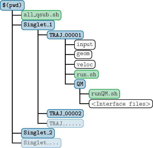
setup_traj.py will create for each initial state a directory where all trajectories starting in this state will be put. If the initial conditions file specified that the initial conditions are in the MCH representation, then the initial states will be assumed to be in the MCH representation as well. In this case, the directories will be named Singlet_0, Singlet_1, …, Doublet_0, Triplet_1, … If the initial states are in the diagonal representation, then the directories are simply called X_1, … since they do not have a definite spin.
In each directory, subdirectories called TRAJ_%05i are created, where %05i is the initial condition index, padded to 5 digits with zeroes. In each trajectory’s directory, an SHARC input file called input will be created, which contains all the dynamics options chosen during the setup_traj.py run. Also, files geom and veloc will be created. For trajectories setup with setup_traj.py, the determination of the initial wave function coefficients is done by SHARC.
If explicitly present, the start time of each trajectory is written into a file start.time in each directory, so that the trajectory can be shifted in time during analysis.
Furthermore, in each trajectory directory a subdirectory QM is created, where the runQM.sh script containing the call to the interface is put (if using sharc.x. In the directory QM also all interface-specific input files will be copied.
For each trajectory, a run.sh script will be created, which can be executed to run the dynamics simulation. You might need to adapt the run script to your cluster setup.
setup_traj.py also creates a script all_run_traj.sh, which can be used to execute all trajectories sequentially.
Note that this is intended for small test trajectories, and should not be used for expensive production trajectories.
For the latter, setup_traj.py can optionally create a script all_qsub_traj.sh, which can be executed to submit all trajectories to a queueing system. You might need to adapt also this script to your cluster setup.
The full directory structure created by setup_traj.py is given in figure 7.2.
7.19 File transfer: retrieve.sh
In some cases, SHARC will run on some temporary directory, and not in the directory where the trajectories have been submitted from. The shell script retrieve.sh is a simple scp wrapper, which can be executed (in a directory where a trajectory has been sent from) in order to retrieve the output files of this trajectory. This might not work for every cluster setup.
It relies on the presence of the file host_infos. All trajectories set up with setup_traj.py create this file after the trajectory has been started with run.sh. retrieve.sh reads host_infos to determine the hostname and working directory of the trajectory and then uses scp to retrieve the output and restart files.
The script can be called with the option “-lis” in order to only retrieve the output.lis file, but not the other output files.
If the script is called with the option “-res” then also the restart files and the content of the restart/ directory are copied.
It is advisable to configure public-key authentification for the hosts running the trajectories, so that not for every execution of retrieve.sh a password has to be entered.
7.20 Resetting trajectories: clean_traj.sh
Especially when developing and when performing preliminary test trajectories, it is useful to quickly reset a trajectory, in order to run it again.
This is especially important because the SHARC drivers will refuse to run a trajectory from time zero if restart files are present.
Similarly, most interfaces will raise an error if interface-specific restart files are present that do not match the requested time step.
The tool clean_traj.sh removes all output and restart files, the output_data/ folder, and empty marker files (STOP, CRASHED, DONT_ANALYZE, RUNNING, DEAD).
Additionally, it recursively removes files from the QM/ and restart/ directories.
7.20.1 Usage
Within a TRAJ_%05i/ folder, simply call the script.
If the script is executed in a directory that does not match this naming convention, it will exit without deleting.
7.21 Ensemble Diagnostics Tool: diagnostics.py
The purpose of this script is to automatize the critical step of checking the trajectories in an ensemble for sanity before beginning the ensemble analysis.
The tool can check several different aspects of the trajectories.
First, it checks whether all relevant output files of the trajectories are present, and if they are complete and consistent (e.g., no missing lines due to network/file system problems).
Second, it checks simulation progress and status (e.g., whether the trajectory is running, crashed, finished, or stopped).
Third, it can check several energy-related requirements: total energy conservation, smoothness of kinetic and potential energy, and hopping energy differences.
It also checks for conservation of total population, and for trajectories using local diabatization also intruder states are checked.
Note that the diagnostics script can also be used to automatically run the data_extractor.x for all trajectories.
Also note that diagnostics.py will not work if the printlevel in the SHARC trajectories was lower than 2.
7.21.1 Usage
The script is interactive, simply start it with no command-line arguments or options:
user@host> $SHARC/diagnostics.py
7.21.2 Input
Paths to trajectories
First the script asks the user to specify all directories for whose content the analysis should be performed. Enter one directory path at a time, and finish the directory input section by typing “end“. Please do not specify each trajectory directory separately, but specify their parent directories, e.g. the directories Singlet_1 and Singlet_2. diagnostics.py will automatically include all trajectories contained in these directories.
Unlike the ensemble analysis scripts (these are populations.py, transition.py, crossing.py, trajana_essdyn.py, trajana_nma.py, and data_collector.py, see below), diagnostics.py ignores files which indicate the status of a trajectory (CRASHED, RUNNING, DONT_ANALYZE) and carries out the diagnostics routines as long as it identifies a directory as a SHARC trajectory.
Settings
The settings for the diagnostics run can be modified with a simple menu, which can be navigated with the commands show, help, end, and where the settings can be modified with <key> <value> (e.g., hop_energy 0.2 sets the corresponding option to 0.2 eV).
A list of the settings is given in Table 7.10.
Generally, the keywords missing_output, missing_restart, and normal_termination should always be left at True, since checking them is cheap and the obtained information is important.
Note that data_extractor.x or data_extractor_NetCDF.x is always run for all trajectories, except if output.dat is older than the files in output_data/.
During the check of each trajectory, output.lis, output_data/energies.out, and output_data/coeff_diag.out are furthermore checked for missing time steps.
| Key | Value | Explanation |
| missing_output | Boolean | Checks if öutput.lis”, öutput.log”, öutput.xyz”, öutput.dat” are existing. Setting to False only suppresses output, but files are always checked. |
| missing_restart | Boolean | Checks if “restart.ctrl”, “restart.traj”, “restart/” are existing. Files are not checked if set to False. |
| normal_termination | Boolean | Checks for status of trajectory: |
| RUNNING: no finish message in output.log, last step started recently. | ||
| STUCK: no finish message in output.log, last step started long ago. | ||
| CRASHED: error message in output.log. | ||
| FINISHED: finish message in output.log. | ||
| FINISHED (stopped by user): finished due to STOP file. | ||
| etot_window | Float | Maximum permissible drift (along full trajectory) in the total energy (in eV). |
| etot_step | Float | Maximum permissible total energy difference between two successive time steps (in eV). |
| epot_step | Float | Maximum permissible active state potential energy difference between two successive time steps (in eV). Not checked for time steps where a hop occurred. |
| ekin_step | Float | Maximum permissible kinetic energy difference between two successive time steps (in eV). |
| pop_window | Float | Maximum permissible drift in total population. |
| hop_energy | Float | Maximum permissible change in active state energy during a surface hop (in eV). |
| intruders | Boolean | Checks if intruder state messages in öutput.log” refer to active state. |
| always_update | Boolean | Run the data_extractor.x always, even if output.dat is older than the produced files. |
| extractor_mode | String | Controls command line flags for the data_extractor.x: |
| xs: Uses the -xs flag. | ||
| s: Uses the -s flag. | ||
| l: Uses the -l flag. | ||
| xl: Uses the -xl flag. | ||
| dont: data_extractor.x is never run (this leads to incomplete diagnostics, but is very fast). |
Trajectory Flagging
diagnostics.py determines for each trajectory a “maximum usable time” value (Tmu).
This value is either the total simulation time or the time when the first violation (problems with time step consistency, total energy conservation, potential/kinetic energy smoothness, hopping energy restriction, or intruder states) in the trajectory appeared.
The script prints the Tmu values for all trajectories at the end.
The user can then give a threshold for Tmu, so that diagnostics.py excludes all trajectories with values smaller than the threshold from analysis (the script will create a file DONT_ANALYZE in the directory of each affected trajectory).
In this way it is possible to perform ensemble analysis for a given simulation length while ignoring problematic trajectories.
When choosing the threshold for Tmu, keep in mind that a compromise usually has to be made.
A small value of the threshold will mean that many trajectories are admitted for analysis (because problems occurring late do not matter), giving good statistics, but that the analysis can only be carried out for the first part of the simulation time.
On the other hand, choosing a large threshold allows analysis of a satisfactory simulation time, but only few trajectories will be included in the analysis (only the ones where no problems occurred for many time steps).
It is advisable that the chosen threshold value is used as input for the ensemble analysis scripts which ask for a maximum analysis time (populations.py, transition.py, crossing.py, trajana_essdyn.py, trajana_nma.py).
7.22 Data Extractor: data_extractor.x
The data_extractor.x is the primary tool to extract useful, tabular data from the output.dat file that is produced by sharc.x.
The produced files can then be further processed, e.g., by plotting them or by computing ensemble statistics with data_collector.py (section 7.36).
7.22.1 Usage
The data_extractor.x is a command line tool, and is called with the output.dat file as an argument, and possibly with some options.
user@host> $SHARC/data_extractor.x [options] output.dat
The program will create a directory output_data/ in the current working directory (not necessarily in the directory where output.dat resides). In this directory, several files are written, containing, e.g., the potential energies depending on time, populations depending on time, etc.
Which files are created can be controlled with the command line options, which are summarized in Table 7.11. For most applications, using the -xs or -s flags should be sufficient.
The default is equivalent to -s.
Note that some options might not be available if the necessary data is not written to output.dat (see write options in Table 4.1).
The program will extract the complete output.dat file until it reaches the EOF.
If a file called start.time is present in the present directory, it is read and the contained time shift is applied to all time steps.
The start.time is present if trajectories were generated with the EOE or PDA excitation schemes.
If you have a start.time file but do not want to apply it, rename the start.time file before running data_extractor.x.
The data_extractor.x program will automatically detect the format of the output.dat file (the SHARC1 release had a different file format than the more recent SHARC2, SHARC3, and SHARC4 releases).
Note that diabatic coefficients can only be obtained if wave function overlaps are present in output.dat.
Furthermore, the data file must contain all time steps, so diabatic coefficients will be wrong if the output_data_steps keyword is used to suppress writing of some time steps.
If you are interested in diabatic populations averaged over an ensemble, some special steps need to be taken.
The reason is that, by default, data_extractor.x equates the diabatic basis with the electronic states as provided in the first time step of the trajectory.
Hence, different trajectories have different diabatic bases and averages across several trajectories are meaningless.
In order to provide a common basis, run the initial condition calculations (using setup_init.py) with reference overlaps.
The resulting QM.out file will then contain the overlaps between the states at the equilibrium geometry and the initial geometry.
The QM.out file can then be provided to data_extractor.x:
user@host:traj/Singlet_2/TRAJ_00123> ln -s init/ICOND_00123/ Reference
user@host:traj/Singlet_2/TRAJ_00123> $SHARC/data_extractor.x output.dat
data_extractor.x will attempt to find and open a file called Reference/QM.out and extract the wave function overlaps from there.
These are then used to define the diabatic basis.
7.22.2 Output
After the program finishes, the directory output_data/ contains a number of files. In each file, the number of columns is dependent in the total number n of states i ∈ {1…n}. The content of the files is listed in Table 7.12.
The file expec.out contains the information of energy.out, spin.out and fosc.out in one file. The content of expec.out can be conveniently plotted by using make_gnuscript.py (section 7.27) to generate a GNUPLOT script.
| Option | Description | Default |
| -h | Display help message and quit. | – |
| -f | File name (file name can also be given without -f) | File name must be given |
| -sk | skip parsing of geom., vel., grad., NAC. | True |
| -xyz | Regenerate output.xyz from output.dat | False |
| -e | Write energy.out | True |
| -d | Write fosc.out | True |
| -da | Write fosc_act.out | True |
| -sp | Write spin.out | True |
| -cd | Write coeff_diag.out, coeff_class_diag.out, coeff_mixed_diag.out |
True |
| -cm | Write coeff_MCH.out, coeff_class_MCH.out, coeff_mixed_MCH.out |
True |
| -cb | Write coeff_diab.out, coeff_class_diab.out, coeff_mixed_diab.out |
True (if overlaps present) |
| -p | Write prob.out | True |
| -x | Write expec.out | True |
| -xm | Write expec_MCH.out | True |
| -id | Write ion_diag.out | False |
| -im | Write ion_MCH.out | False |
| -dd | Write dip_mom_diag.out | False |
| -dm | Write dipoles_diag.out, dipoles_MCH.out | False |
| -xs | -e, -d, -cd, m, -p, -x | |
| -s | -sp, -xm, -cb, -da, -dm plus -xs | Default |
| -l | -id, -im plus -s | |
| -xl | -dd plus -l (i.e., all) |
|
Table 7.12: Content of the files written by data_extractor.x. n is the total number of states, j is a state index (j ∈ {1..n}), and α is the active state.
|
||||
| File | # Columns | Columns | ||
|
energy.out |
4+n | 1 | Time t (fs) | |
| 2 | Kinetic energy (eV) | |||
| 3 | Potential energy (eV) of active state (diagonal) | |||
| 4 | Total energy (eV) | |||
| 4+j | Potential energy (eV) of state j (diagonal) | |||
| fosc.out | 2+n | 1 | Time t (fs) | |
| 2 | Oscillator strength from lowest to active state (diagonal) | |||
| 2+j | Oscillator strength from lowest state to state j (diagonal) | |||
| fosc_act.out | 1+2n | 1 | Time t (fs) | |
| 1+j | Ej−Eactive (in eV, diagonal) | |||
| 1+n+j | Oscillator strength from active state to state j (diagonal) | |||
| spin.out | 2+n | 1 | Time t (fs) | |
| 2 | Total spin expectation value of active state | |||
| 2+j | Total spin expectation value of state j | |||
| coeff_diag.out | 2+2n | 1 | Time t (fs) | |
| 2 | Norm of wave function ∑j |cjdiag|2 | |||
| 1+2j | ℜ(cjdiag) | |||
| 2+2j | ℑ(cjdiag) | |||
| coeff_class_diag.out | 2+n | 1 | Time t (fs) | |
| 2 | 1 | |||
| 2+j | δjα | |||
| coeff_mixed_diag.out | 2+n | 1 | Time t (fs) | |
| 2 | 1 | |||
| 2+j | δjα | |||
| coeff_MCH.out | 2+2n | 1 | Time t (fs) | |
| 2 | Norm of wave function ∑j |cjMCH|2 | |||
| 1+2j | ℜ(cjMCH) | |||
| 2+2j | ℑ(cjMCH) | |||
| coeff_class_MCH.out | 2+n | 1 | Time t (fs) | |
| 2 | 1 | |||
| 2+j | |Ujα|2 | |||
| coeff_mixed_MCH.out | 2+n | 1 | Time t (fs) | |
| 2 | 1 | |||
| 2+j | |Ujα|2+∑k,l2ℜ(UjkU*jlcdiagkcdiag*l) | |||
| coeff_diab.out | 2+2n | 1 | Time t (fs) | |
| 2 | Norm of wave function ∑j |cjdiab|2 | |||
| 1+2j | ℜ(cjdiab) | |||
| 2+2j | ℑ(cjdiab) | |||
| coeff_class_diab.out | 2+2n | 1 | Time t (fs) | |
| 2 | 1 | |||
| 2+j | |Tjα|2 | |||
| coeff_mixed_diab.out | 2+2n | 1 | Time t (fs) | |
| 2 | 1 | |||
| 2+j | |Tjα|2+∑k,l2ℜ(TjkT*jlcdiagkcdiag*l) | |||
| prob.out | 2+n | 1 | Time t (fs) | |
| 2 | Random number from surface hopping | |||
| 2+j | Cumulated hopping probability ∑k=1j Pk | |||
| expec.out | 4+3n | 1 | Time t (fs) | |
| 2 | Kinetic energy (eV) | |||
| 3 | Potential energy (eV) of active state (diagonal) | |||
| 4 | Total energy (eV) | |||
| 4+j | Potential energy (eV) of state j (diagonal) | |||
| 4+n+j | Total spin expectation value of state j (diagonal) | |||
| 4+2n+j | Oscillator strength of state j (diagonal) | |||
| expec_MCH.out | 4+3n | 1 | Time t (fs) | |
| 2 | Kinetic energy (eV) | |||
| 3 | Potential energy (eV) of approximate active state (MCH) | |||
| 4 | Total energy (eV) | |||
| 4+j | Potential energy (eV) of state j (MCH) | |||
| 4+n+j | Total spin expectation value of state j (MCH) | |||
| 4+2n+j | Oscillator strength of state j (MCH) | |||
| ion_diag.out | 4+3n | 1 | Time t (fs) | |
| 1+j | Ej−Eactive (in eV, diagonal) | |||
| 1+n+j | Dyson norm from active state to state j (diagonal) | |||
| ion_MCH.out | 4+3n | 1 | Time t (fs) | |
| 1+j | Ej−Eapproximate active (in eV, MCH) | |||
| 1+n+j | Dyson norm from approximate active state to state j (MCH) | |||
| dip_mom_diag.out | Formatted like a minimal output.dat | |||
| file containing the dipole moment matrices | ||||
| in diagonal representation. | ||||
| dipoles_diag.out | 2+n | 1 | Time t (fs) | |
| 2 | Static dipole moment of active state (Debye, diagonal) | |||
| 2+j | Static dipole moment of state j (Debye, diagonal) | |||
| dipoles_MCH.out | 2+n | 1 | Time t (fs) | |
| 2 | Static dipole moment of active state (Debye, MCH) | |||
| 2+j | Static dipole moment of state j (Debye, MCH) | |||
7.23 Data Extractor for NetCDF: data_extractor_NetCDF.x
This program has the same function as the data_extractor.x.
While the latter acts on ASCII-formatted output.dat files, the data_extractor_NetCDF.x reads only the header from output.dat, but the time step data from output.dat.nc.
This file is obtained by setting output_format to ascii in the SHARC input file.
For more details, see Section 5.4.
If a file called start.time is present in the present directory, it is read and the contained time shift is applied to all time steps.
The start.time is present if trajectories were generated with the EOE or PDA excitation schemes.
If you have a start.time file but do not want to apply it, rename the start.time file before running data_extractor_NetCDF.x.
Note that this program currently does not support a few options of the data_extractor.x.
In particular, the options -sk, -dd, -id, and -im are ignored and no corresponding output is produced.
Using the -xyz flag, the data_extractor_NetCDF.x can be used to write an output.xyz file from the NetCDF data file.
7.23.1 Usage
The data_extractor_NetCDF.x is used in the same way as data_extractor.x:
user@host> $SHARC/data_extractor_NetCDF.x [options] output.dat
Note that both output.dat and output.dat.nc need to be present.
The file name of output.dat.nc is hardcoded, if your file is called differently, you should set a symbolic link.
7.23.2 Output
Same as data_extractor.x.
7.24 Data Converter for NetCDF: data_converter.x
This program can be used to convert an output.dat file into a NetCDF file (output.dat.nc).
This significantly reduces the size of the file, and allows deleting the output.xyz file (its content will be in the NetCDF file).
7.24.1 Usage
The data_converter.x usage is very simple:
user@host> $SHARC/data_converter.x output.dat
Note that the data_converter.x does not modify the output.dat file.
Hence, in order to save disk space, remove the data (below the header) afterwards:
user@host> sed -i '1,/End of header array data/!d' output.dat
7.24.2 Output
The program writes a file called output.dat.nc.
This file can be extracted as usual with data_extractor_NetCDF.x (see Section 7.23).
7.25 Data Converter from NetCDF to ASCII: data_converter_to_ASCII.x
This program converts a output.dat.nc to output.dat.cp, which will be in ASCII format.
This will blow up the file size, but is sometimes necessary or convenient for the inspection of the file content or to apply certain scripts.
7.25.1 Usage
The data_converter_to_ASCII.x usage is very simple, and fully analogous to data_extractor_NetCDF.x:
user@host> $SHARC/data_converter_to_ASCII.x output.dat
Note that both output.dat and output.dat.nc need to be present.
The file name of output.dat.nc is hardcoded, if your file is called differently, you should set a symbolic link.
7.25.2 Output
The program writes a file called output.dat.cp.
This file can be extracted as usual with data_extractor.x (see Section 7.22).
7.26 Data Converter from NetCDF nuclear files to XYZ: data_extractor_NUC_xyz.py
If the option output_format ascii_separate_nuclei is used, then the nuclear coordinates end up in the file output_NUC.dat.nc.
This file cannot be extracted by data_extractor_NetCDF.x -xyz to produce an xyz file for analysis.
However, using data_extractor_NUC_xyz.py, the xyz file can be generated.
7.26.1 Usage
Usage is very simple:
user@host> python $SHARC/data_extractor_NUC_xyz.py geom output_NUC.dat.nc > output_NM.xyz
Note that the script reads the element symbols from the geom file.
The script can read either output_NUC.dat.nc or output.dat.nc.
7.26.2 Options
The script has only one option, -q STR.
The given string (recommended in quotes) gives a list of the atoms to extract.
For example, -q "1 8 21 28" creates an XYZ file containing 16 atoms, which are taken from atoms 1-8 and 21-28 from the NetCDF file.
7.26.3 Output
The program writes the xyz coordinates to standard output.
Redirect the output to store it in a file.
7.27 Plotting the Extracted Data: make_gnuscript.py
The contents of the output files of data_extractor.x can be plotted with GNUPLOT. In order to quickly generate an appropriate GNUPLOT script, make_gnuscript.py can be used. The usage is:
user@host> $SHARC/make_gnuscript.py <S> [<D> [<T> [<Q> ... ] ] ]
make_gnuscript.py takes between 1 and 8 integers as command-line arguments, specifying the number of singlet, doublet, triplet, etc. states. It writes an appropriate GNUPLOT script to standard out, hence redirect the output to a file, e.g.:
user@host> $SHARC/make_gnuscript.py 3 0 2 > gnuscript.gp
Then, GNUPLOT can be run in the output_data directory of a trajectory:
user@host> gnuplot gnuscript.gp
This can also be accomplished in one step using a pipe, e.g.:
user@host> $SHARC/make_gnuscript.py 3 0 2 | gnuplot
The created plot script generates four different plots (press ENTER in the command-line where you started GNUPLOT to go to the next plot). The first plot shows the potential energy of all states in the dynamics over time in the diagonal representation. The currently occupied state is marked with black circles. A thin black line gives the total energy (sum of the kinetic energy and the potential energy of the currently occupied state). Each state is colored, with one color as contour and one color at the core of the line. The contour color represents the total spin expectation value of the state. The core color represents the oscillator strength of the state with the lowest state. See figure 7.3 for the relevant color code.
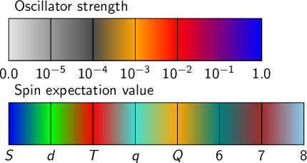
Note that by definition the “oscillator strength” of the lowest state with itself is exactly zero, hence the lowest state is also light grey. This dual coloring allows for a quick recognition of different types of states in the dynamics, e.g. singlets vs. triplets or nπ* vs. ππ* states.
The second plot shows the same data again, but using relative energies such that the energy of the lowest state is zero.
The third plot shows the population |ciMCH|2 of the MCH electronic states over time. The line colors are auto-generated in order to give a large spread of all colors over the excited states, but the colors might be sub-optimal, e.g. for printing. In this cases, the user should manually adjust the colors in the generated script.
The fourth plot shows the population |cidiag|2 of the diagonal electronic states over time. These are the populations which are actually used for surface hopping. However, since these states are spin-mixed, it is usually difficult to interpret these populations.
The fifth plot shows the surface hopping probabilities over time. The plot is setup in such a way that the visible area corresponding to a certain state is proportional to the probability to hop into the state. Hence, if for a given time step the random number (black circles) lies within a colored area, a surface hop to the corresponding state is performed.
7.28 Internal Coordinates Analysis: geo.py
SHARC writes at every time step the molecular geometry to the file output.xyz. The non-interactive script geo.py can be used in order to extract internal coordinates from xyz files. The usage is:
user@host> $SHARC/geo.py [options] < Geo.inp > Geo.out
By default, the coordinates are read from output.xyz, but this can be changed with the -g option (see table 7.14). Note that the internal coordinate specifications are read from standard input and the result table is written to standard out.
If a file called start.time is present in the present directory, it is read and the contained time shift is applied to all time steps.
The start.time is present if trajectories were generated with the EOE or PDA excitation schemes.
If you have a start.time file but do not want to apply it, use the -ignore_start_time option.
If a starting time step is set manually with -T, then the start.time file is ignored.
Note that the time shift from start.time must be compatible with the time step given via -t.
7.28.1 Input
The specifications for the desired internal coordinates are read from standard input. It follows a simple syntax, where each internal coordinate is specified by a single line of input. Each line starts with a one-letter key which specifies the type of internal coordinate (e.g. bond length, angle, dihedral, …). The key is followed by a list of integers, specifying which atoms should be measured. As a simple example, r 1 2 specifies the bond length (r is the key for bond lengths) between atoms 1 and 2. Note that the numbering of the atoms starts with 1. Each line of input is checked for consistency (whether any atom index is larger than the number of atoms, repeated atom indices, misspelled keys, wrong number of atom indices, …), and erroneous lines are ignored (this is indicate by an error message).
Table 7.13 lists the available types of internal coordinates. The output is a table, where the first column is the time (Actually, the geometries are just enumerated starting with zero, and the number multiplied by the time step from the -t option). The successive columns in the output table list the results of the internal coordinates calculations. Each request generates at least one column, see table 7.13.
Note that for most internal coordinates, the order of the atoms is crucial, since e.g. a123 ≠ a213. This also holds for the Cremer-Pople parameter requests. For these input lines, the atoms should be listed in the order they appear in the ring (clockwise or counter-clockwise).
| Key | Atom | Description | Output columns |
| Indices | |||
| x | a | x coordinate of atom a | x |
| y | a | y coordinate of atom a | y |
| z | a | z coordinate of atom a | z |
| r | a b | Bond length between a and b | r |
| a | a b c | Angle between a–b and b–c | a |
| d | a b c d | Dihedral, i.e., angle between normal vectors of (a,b,c) and (b,c,d) | d |
| (between -180° and 180°, same sign conventions as MOLDEN) | |||
| p | a b c d | Pyramidalization angle: 90° minus angle between bond a–b | p |
| and normal vector of (b,c,d) | |||
| q | a b c d | Pyramidalization angle (alternative definition; angle between | q |
| bond a–b and average of bonds b–c and b–d | |||
| 5 | a b c d e | Cremer-Pople parameters for 5-membered rings [66] and | q2, ϕ2, Boeyens |
| comformation classification. | |||
| 6 | a b c d e f | Cremer-Pople parameters for 6-membered rings [66] and | Q, ϕ, θ, Boeyens |
| Boeyens classification [67]. | |||
| i | a – f | Angle between average plane through 3-rings (a - c) and (d - f) | i |
| j | a – h | Angle between average plane through 4-rings (a - d) and (e - f) | j |
| k | a – j | Angle between average plane through 5-rings (a - e) and (f - j) | k |
| l | a – l | Angle between average plane through 6-rings (a - f) and (g - l) | l |
| c | Writes the comment (second line of the | Comment | |
| xyz format) to the table. |
As an advice, it is always a good idea to put the comment as the last request, if needed. Since the comment may contain blanks, having the comment not as the very last column might make it impossible to plot the resulting table.
The Boeyens classification symbols which are output for 6-membered rings are reported in LATEX math code. Note that in the Boeyens classification scheme by definition a number of symbols are equivalent, and only one symbol is reported.
These are the equivalent symbols: 1C4=3C6=5C2, 4C1=6C3=2C5, 1T3=4T6, 2T6=5T3, 2T4=5T1, 3T1=6T4, 6T2=3T5 and 4T2=1T5.
For 5-membered rings, the classification symbols are chosen similar to the Boeyens symbols. For the aE and Ea symbols, atom a is puckered out of the plane and the four other atoms are coplanar, while for the aHb symbols the neighboring atoms a and b are puckered out of the plane in opposite directions and only the three remaining atoms are coplanar.
It is also possible to measure angles between the average planes through two n-membered rings.
Currently, this is only possible if both rings have the same number of atoms (3, 4, 5, or 6).
7.28.2 Options
geo.py accepts a number of command-line options, see table 7.14. All options have sensible defaults. However, especially if long comments should be written to the output file, it might be necessary to increase the field width. Note that the minimum column width is 20 so that the table header can be printed correctly.
Also note that the column for the comment is enlarged by 50 characters.
| Option | Description | Default |
| -h | Display help message and quit. | – |
| -b | Report x, y, z, r, q2 and Q in Bohrs | Angstrom |
| -r | Report a, d, p, q, ϕ2, ϕ, θ, i, j, k, and l in Radians | Degrees |
| -g FILENAME | Read coordinates from the specified file | output.xyz |
| -t FLOAT | Assumed time step between successive geometries (fs) | 1.0 fs |
| -w INTEGER | Width of each column (min=20) | 20 |
| -p INTEGER | Precision (Number of decimals, min=width-3) | 4 |
| -T INTEGER | Start counting time step | 0 |
| -ignore_start_time | Do not apply shift from start.time | include shift |
| -n | Pad with NaNs between 0 fs and first time step (with -T or start.time | File starts later |
7.29 Normal Mode Analysis: geo_NM.py
The non-interactive script geo_NM.py computes normal mode coordinates for a given molecular trajectory.
The usage is:
user@host> $SHARC/geo_NM.py [options] > Geo_NM.out
By default, the coordinates are read from output.xyz, but this can be changed with the -g option (see Table 7.15).
Additionally, the normal mode definitions are read from the V0.txt file, which contains the parameters defining the normal mode coordinates.
The result table is written to standard output.
The computation uses the same formulae as for SHARC_LVC.py when computing the normal mode coordinates (Equation (8.108)).
If a file called start.time is present in the present directory, it is read and the contained time shift is applied to all time steps.
The start.time is present if trajectories were generated with the EOE or PDA excitation schemes.
If you have a start.time file but do not want to apply it, use the -ignore_start_time option.
If a starting time step is set manually with -T, then the start.time file is ignored.
Note that the time shift from start.time must be compatible with the time step given via -t.
7.29.1 Input
Table 7.15 lists the available options for the script.
| Option | Description | Default |
| -h | Display help message and quit. | – |
| -p | Number of decimals for normal mode coordinates | 4 |
| -w | Field width for the output table | 20 |
| -g FILENAME | Read coordinates from the specified geometry file | output.xyz |
| -v FILENAME | Use the specified file with normal mode definitions | V0.txt |
| -t FLOAT | Timestep between successive geometries in fs | 1.0 |
| -T INTEGER | Start counting the timesteps from a specified value | 0 |
| -k | Switch on aligning the structures using the Kabsch algorithm | off |
| -q STRING | Specify list of considered atoms for normal mode calculation (e.g., “18 12 20”) | all atoms |
| -b | Enable buffered reading of the geometry file (useful for large files) | off |
| -n | Pad with NaNs between 0 fs and first time step (with -T or start.time | File starts later |
Using the options -k and -q, one can analyze the normal mode coordinates of a subsystem of a large calculation, e.g., a QM/MM calculation.
Use the -q option to select which atoms are considered for the normal mode computation.
The number of selected atoms must match the atom number in the V0.txt file.
Turn on the -k option in case the molecule/selected atoms have not the same orientation as the reference geometry (which is generally the case in QM/MM calculations), so that the geometry is aligned prior to computing the normal mode coordinates.
7.29.2 Output Format
The output is a table where each row corresponds to a geometry snapshot in the trajectory. The first column contains the time in femtoseconds, and the following columns contain the normal mode coordinates for each mode. The last column contains the comment from the geometry file.
| Time (fs) | Mode 1 | Mode 2 | … | Comment |
| 0.00 | 0.123456 | 0.234567 | … | First snapshot |
| 1.00 | 0.234567 | 0.345678 | … | Second snapshot |
| Mode | Description | From which file? | Extract? |
| 1 | For each diagonal state count how many trajectories have this state as active state. | output.lis | No |
| 2 | For each MCH state count how many trajectories have this state as approximate active state (see section 8.23.1). | output.lis | No |
| 3 | For each MCH state count how many trajectories have this state as approximate active state (see section 8.23.1). Multiplet components are summed up. | output.lis | No |
| 4 | Generate a histogram with definable bins (variable width). Bin the trajectories according to their total spin expectation value (of the currently active diagonal state). | output.lis | No |
| 5 | Generate a histogram with definable bins (variable width). Bin the trajectories according to their state dipole moment expectation value (of the currently active diagonal state). | output.lis | No |
| 6 | Generate a histogram with definable bins (variable width). Bin the trajectories according to the oscillator strength between lowest and currently active diagonal states. | output_data/fosc.out | Yes |
| 7 | Calculate the sum of the absolute squares of the diagonal coefficients for each state. | output_data/coeff_diag.out | Yes |
| 8 | Calculate the sum of the absolute squares of the MCH coefficients for each state. | output_data/coeff_MCH.out | Yes |
| 9 | Calculate the sum of the absolute squares of the MCH coefficients for each state. Multiplet components are summed up. | output_data/coeff_MCH.out | Yes |
| 12 | Transform option 1 to MCH basis (section 8.5). | output_data/coeff_class_MCH.out | Yes |
| 13 | Transform option 1 to MCH basis (section 8.5). Multiplet components are summed up. | output_data/coeff_class_MCH.out | Yes |
| 14 | Wigner-transform option 1 to MCH basis (section 8.5). | output_data/coeff_mixed_MCH.out | Yes |
| 15 | Wigner-transform option 1 to MCH basis (section 8.5). Multiplet components are summed up. | output_data/coeff_mixed_MCH.out | Yes |
| 20 | Calculate the sum of the absolute squares of the diabatic coefficients for each state (Only for trajectories with local diabatization). | output_data/coeff_diab.out | Yes |
| 21 | Transform option 1 to diabatic basis (section 8.5). | output_data/coeff_class_diab.out | Yes |
| 22 | Wigner-transform option 1 to diabatic basis (section 8.5). Multiplet components are summed up. | output_data/coeff_mixed_diab.out | Yes |
Run data extractor
For analysis modes 6, 7, 8, 9 and 20 it is necessary to first run the data extractor (see Section 7.22 or Section 7.23).
The script automatically detects whether the regular or NetCDF extractor should be called.
This task can be accomplished by populations.py. However, for a large ensemble or for long trajectories this may take some time. Hence, it is not necessary to perform this step each time populations.py is run.
populations.py will detect whether the file output.dat or the content of output_data/ is more recent. Only if output.dat is newer the data_extractor.x will be run for this trajectory.
Note that mode 20 can only be used for trajectories using local diabatization propagation (keyword coupling overlap in SHARC input file) or .
Number of states
For analysis modes 1, 2, 3, 7, 8 and 9 it is necessary to specify the number of states in each multiplicity. The number is auto-detected from the input file of one of the trajectories.
Intervals
For analysis modes 4, 5 and 6 the user must specify the intervals (i.e., the histogram bins) for the classification of the trajectories. The user has to input a list of interval borders, e.g.:
Please enter the interval limits, all on one line.
Interval limits: 1e-3 0.01 0.1 1
Note that scientific notation can be used. Based on this input, for each time step a histogram is created with the number of trajectories in each interval. The histogram bins are:
- x ≤ 10−3
- 10−3 < x ≤ 0.01
- 0.01 < x ≤ 0.1
- 0.1 < x ≤ 1
- 1 < x
Note that there is always one more bin that interval borders entered.
Normalization
If desired, populations.py can normalize the populations by dividing the populations by the number of trajectories.
Maximum simulation time
This gives the maximum simulation time until which the populations are analyzed. For trajectories which are shorter than this value, the last population information is used to make the trajectory long enough. Trajectories which are longer are not analyzed to the end. populations.py prints the length of the shortest and longest trajectories after the analysis.
If diagnostics.py was executed previously, the user can enter here the threshold for the maximum usable time (see section 7.21).
Setup for bootstrapping
The output file of populations.py is sufficient to perform kinetic model fits with the script make_fitscript.py.
However, if error estimates for the kinetic model are desired (using bootstrap.py), the output file of populations.py is not enough.
The user can tell populations.py to save additional data which is required by bootstrap.py.
Gnuplot script
populations.py can generate an appropriate GNUPLOT script for the performed population analysis.
7.31.2 Output
By default, populations.py writes the resulting populations to pop.out. If the file already exists, the user is ask whether it shall be overwritten, or to provide an alternative filename. Note that the output file is checked only after the analysis is completed, so the program might run for a considerable amount of time before asking for the output file.
If files start.time are present in the trajectory folders, the contained time shift is automatically applied to each trajectory.
7.32 Calculation of Numbers of Hops: transition.py
Another important information from the trajectory ensemble is the number of hopping events and the involved states, for example to judge the relative importance of competing reaction pathways.
The interactive script transition.py calculates from an ensemble the number of hops between each pair of states and presents the results as “transition matrices”.
Currently, the script employs the MCH active state information from output.lis for this computations.
Note that since the MCH active state is only an approximate quantity (since hops are actually performed in the diagonal basis in SHARC), the results should be checked carefully.
The script transition.py is still partly work-in-progress.
7.32.1 Usage
The script is interactive, simply start it with no command-line arguments or options:
user@host> $SHARC/transition.py
Paths to trajectories
First the script asks the user to specify all directories for whose content the analysis should be performed. Enter one directory path at a time, and finish the directory input section by typing “end“. Please do not specify each trajectory directory separately, but specify their parent directories, e.g. the directories Singlet_1 and Singlet_2. populations.py will automatically include all trajectories contained in these directories.
If you want to exclude certain trajectories from the analysis, it is sufficient to create an empty file called CRASHED or RUNNING in the corresponding trajectory directory. populations.py will ignore all directories containing one of these files. The file name is case insensitive, i.e., also files like crashed or even cRasHED will lead to the trajectory being ignored.
Additionally, transition.py will ignore trajectories with a DONT_ANALYZE file from diagnostics.py.
Analysis mode
The different analysis modes for transition.py are given in Table 7.18.
| Mode | Description | From which | Extract? |
| file? | |||
| 1 | Get transition matrix in MCH basis. | output.lis | No |
| 2 | Get transition matrix in MCH basis, ignoring hops within multiplets. | output.lis | No |
| 3 | Write a tabular file with the transition matrix in the MCH basis for each time step. | output.lis | No |
| 4 | Write a tabular file with the transition matrix in the MCH basis for each time step, ignoring hops within multiplets. | output.lis | No |
7.33 Fitting population data to kinetic models: make_fit.py
Often it is interesting to fit some functions to the population data from a trajectory ensemble, in order to provide a way to abstract the data and to obtain some kind of rate constants for population transfer, which allows to compare to experimental works.
In simple cases, it might be sufficient to fit basic mono- and biexponential functions to the data, which provides the sought-after time constants.
However, often a more meaningful approach is based on a chemical kinetics model.
Such a model is specified by a set of chemical species (e.g., electronic states, reactants, products, etc) connected by elementary reactions with associated rate constants, which together form a reaction network graph.
For an explanation of those graphs, see section 8.10.
The script make_fit.py helps the user in implementing and fitting such global fits to a kinetics model.
The script works in a stand-alone fashion, unlike its predecessors (make_fitscript.py and bootstrap.py).
It solves the differential equations numerically using a Runge-Kutta 5th order algorithm and fits the kinetic parameters using a number of different optimization algorithms.
Often, one is also interested in obtaining an estimate of the error associated to these rate constants, e.g., in order to decide whether enough trajectories were computed.
A possible way to obtain such error estimates is the statistical bootstrapping procedure.
The idea of bootstrapping is to generate resamples of the original ensemble; for an ensemble of n trajectories, one draws n random trajectories with replacement to obtain one resample.
The resample can then be fitted like the original ensemble to obtain a second estimate of the rate constants.
By generating many resamples, one can thus obtain a “probability” distribution of the rate constants, from which a statistical error measure can be calculated.
For details on these statistical measures, see section 8.4.
The script make_fit.py implements this resampling-fitting-statistics procedure.
It is dependent on the output of populations.py, but otherwise works in a stand-alone fashion.
7.33.1 Usage
The script is interactive, simply start it with no command-line arguments or options:
user@host> $SHARC/make_fit.py
Before you start the script, you need to prepare a file with the relevant populations data (usually, the output file of populations.py will suffice).
You also might want to run transition.py first, which can help in developing a suitable kinetic model.
7.33.2 Input
The interactive input for this script consists of specifying the reaction network graph, the initial conditions and the data file.
Additionally, the user has to specify which species should be fitted to which data columns in the file.
Optionally, the user can specify the bootstrap settings for estimating errors.
Kinetic model species
As a first step, the user has to specify the set of species in the model.
Each species is fully described by its label.
A label must start with a letter and can be followed by letters, numbers and underscores (although an underscore must not be directly followed by another underscore).
During input, the user can add one or several labels to the set of species, remove labels and display the current set of defined labels.
It is not possible to add a label twice.
Once all labels are defined, the keyword end brings the user to the next input section (hence, end is not a valid label).
Kinetic model elementary reactions
Next, the reactions have to be defined.
A reaction is specified by its initial species, final species, and reaction rate label.
Reaction rate labels are under the same restrictions as species labels and must not be already used as a species label.
Furthermore, initial and final species must be both defined previously and they must be different.
There can only be one reaction from any species to another species (If a second reaction is defined, the first reaction label is simply overwritten).
Note that reaction rate labels can be used in several reactions (in this way, different rates can be restricted to be the same).
During input, the user can add and remove reactions and display the currently defined reactions (displayed as a matrix).
Unlike species labels, only one reaction can be added per line.
Once all reactions are defined, the keyword end brings the user to the next input section.
Kinetic model initial values
In order to specify the initial values for each species, the user simply has to define which species have non-zero initial population.
These species will then be assigned an initial population constant, which can be fitted along with the reaction rates.
During input, the user can add and remove species from the set of species with non-zero initial population.
Once all reactions are defined, the keyword end brings the user to the next input section.
Operation mode
The script can either read a pop.out file for a simple global fit, or a bootstrap_data/ directory for a global fit with error estimate.
If the latter is chosen, the user needs to enter the number of bootstrap cycles.
Populations data file
The user has to specify a path (autocomplete is enabled) to the file containing the population data to which the model functions should be fitted.
In bootstrap mode, instead the path to the bootstrap_data/ directory (can be prepared with populations.py) needs to be given.
The script reads the file/files and automatically detects the maximum time and the number of data columns.
The file/files should be formatted as a table, with one time step per line (e.g., an output file of populations.py).
On each line, the first number is interpreted as the time in femtoseconds and all consecutive numbers (separated by spaces) as the populations at this time.
Note that the first entry must be at t=0 and all subsequent lines must be in strictly increasing order.
Time steps can be unevenly spaced if necessary.
Species-Data mapping
In the next setup section, the user has to specify which functions should be fitted to which data column from the data file.
In the simplest case, one species is fitted to a single data column (e.g., the species S0 is fitted to data column 2).
However, it is also possible to fit the sum of two species to a column (this can be useful, e.g., to describe biexponential processes) and to fit a species to the sum of several columns (e.g., one can fit to the total triplet population to obtain a total ISC rate constant).
In general, it is also possible to fit sums of species to sums of columns.
It is not allowed to use one species or one column in more than one mapping.
However, it is possible to leave species or data columns unused in the global fit.
While unused species still affect the outcome (through the reaction network definitions), unused data columns are simply ignored in the fit.
During input, the user can add one mapping per line as well as display the current mappings.
For the column definitions, ranges can be given with the tilde symbol, e.g., 5 9 is interpreted as 5 6 7 8 9.
If a typo is made, the user can reset the mappings and repeat only the mapping input without the need to repeat the previous sections.
Once all mappings are defined, the keyword end finishes the input section.
Fitting procedure
In the last section, the user can edit the initial guesses for the rate constants and initial populations.
To change a value, enter label = value.
Use show to print the current values for all constants.
end finishes the guess edit step.
Afterwards, the script asks whether the initial populations should be optimized or not.
This is usually only useful if several species have non-zero initial populations.
If you optimize initial populations, note that their sum might differ from 1 after optimization.
The script also asks whether the rate constants should be constrained to positive values.
If answered with yes, then the optimized rate constants are restricted to the range 0.000 001 to infinity (i.e., the time constants are constrained between 1 000 000 fs and 0 fs).
Note that with constraints SCIPY uses the Trust Region Reflective algorithm, and the Levenberg-Marquardt algorithm for unconstrained cases.
7.33.3 Output
The script will write the output to standard out.
It will first print the iterations of the fit, and the obtained results afterwards (all fitted parameters with errors).
The script will also write two files, fit_results.txt and fit_results.gp.
The latter is a GNUPLOT script that can be used to plot the global fit, which is useful for visual inspection.
Note that the errors printed for normal runs are just the intrinsic fitting errors, which assume that the population data is error-free.
To obtain realistic fitting errors that take into account the uncertainty due to the finite trajectory ensemble, use the bootstrap mode.
In bootstrap mode, the script initially will perform the same steps as in normal mode, using the average population from the bootstrap directory.
After writing the fit results and the two files, the script will start performing the bootstrap iterations, writing the fitted parameters in each iteration.
In this way, the user can monitor the convergence of these values, to decide whether more iterations are required.
Typically, the values and errors will vary strongly during the first iterations and stabilize later.
The convergence rate is strongly dependent on the fitting model and the data.
After all iterations are done (or the script is interrupted with Ctrl-C), the script will print a summary of the statistical analysis.
For each fitting parameter (all time constants and all initial populations), the script will list the arithmetic mean and standard deviation (absolute and relative), the geometric mean and standard deviation (separately for + and −, absolute and relative), and the minimum and maximum values.
The script will also print a histogram with the obtained distribution for each parameter.
For details on these statistical measures, see section 8.4.
bootstrap.py also creates an output file once it is finished.
The file, fit_bootstrap.txt, contains the summary of the statistical analysis with the computed statistical measures and the histograms.
Additionally, at the end this file contains a table with all obtained fitting parameters for resamples (e.g., for further statistical or correlation analysis).
7.34 Obtaining Special Geometries: crossing.py
In many cases, it is also important to obtain certain special geometries from the trajectories. The script crossing.py extracts geometries fulfilling special conditions from an ensemble of trajectories.
Currently, crossing.py finds geometries where the approximate MCH state (see section 8.23.1) of the last time step is different from the MCH state of the current time step (i.e. crossing.py finds geometries where surface hops occured).
7.34.1 Usage
The script is interactive, simply start it with no command-line arguments or options:
user@host> $SHARC/crossing.py
The input to the script is very similar to the one of populations.py.
Paths to trajectories
First the script asks the user to specify all directories for whose content the analysis should be performed. Enter one directory path at a time, and finish the directory input section by typing “end“. Please do not specify each trajectory directory separately, but specify their parent directories, e.g. the directories Singlet_1 and Singlet_2. crossing.py will automatically include all trajectories contained in these directories.
If you want to exclude certain trajectories from the analysis, it is sufficient to create an empty file called CRASHED or RUNNING in the corresponding trajectory directory. crossing.py will ignore all directories containing one of these files.
Additionally, crossing.py will ignore trajectories with a DONT_ANALYZE file from diagnostics.py.
Analysis mode
Currently, crossing.py only supports one analysis mode, where crossing.py is scanning for each trajectory the file output.lis. If the occupied MCH state (column 4 in output file output.lis) changes from one time step to the next, it is checked whether the old and new MCH states are the ones specified by the user. If this is the case, the geometry corresponding to the new time step (t) is retrieved from output.xyz (lines t(natom+2)+1 to t(natom+2)+natom).
States involved in surface hop
First, the user has to specify the permissible old MCH state. The state has to be specified with two integers, the first giving the multiplicity (1=singlet, …), the second the state within the multiplicity (1 1=S0, 1 2=S1, etc.). If a state of higher multiplicity is given, crossing.py will report all geometries where the old MCH state is any of the multiplet components.
For the new MCH state, the same is valid.
Third, the direction of the surface hop has to be specified. Choosing “Backwards” has the same effect as exchanging the old and new MCH states.
7.34.2 Output
All geometries are in the end written to an output file, by default crossing.xyz. The file is in standard xyz format. The comment of each geometry gives the path to the trajectory where this geometry was extracted, the simulation time and the diagonal and MCH states at this simulation time.
7.35 Essential Dynamics Analysis: trajana_essdyn.py
An essential dynamics analysis [70] is a procedure to find the most active vibrational modes in an ensemble of trajectories.
It is based on the computation of the covariance matrix between all Cartesian (or mass-weighted Cartesian) coordinates of all steps of all trajectories and a singular value decomposition of this covariance matrix.
For details on the computation, see section 8.8.
The interactive script trajana_essdyn.py can be used to perform such an analysis.
7.35.1 Usage
trajana_essdyn.py is an interactive script, which is started with:
user@host> $SHARC/trajana_essdyn.py
Note that before executing the script you should prepare an XYZ geometry file with the reference geometry (e.g., the ground state minimum or the average geometry from the trajectories).
7.35.2 Input
During interactive input, the script queries for the paths to the trajectories, the path to the reference structure, and a few other settings.
Path to the trajectories
First the script asks the user to specify all directories for whose content the analysis should be performed. Enter one directory path at a time, and finish the directory input section by typing “end“. Please do not specify each trajectory directory separately, but specify their parent directories, e.g. the directories Singlet_1 and Singlet_2. trajana_essdyn.py will automatically include all trajectories contained in these directories.
If you want to exclude certain trajectories from the analysis, it is sufficient to create an empty file called CRASHED or RUNNING in the corresponding trajectory directory. trajana_essdyn.py will ignore all directories containing one of these files.
Additionally, trajana_essdyn.py will ignore trajectories with a DONT_ANALYZE file from diagnostics.py.
Path to reference structure
For the essential dynamics analysis, a reference structure is required. This structure is substracted from all geometries for the correlation analysis.
The structure can be in any format understandable by OPENBABEL, but the type of format needs to be specified.
In most cases, the reference structure will be either in XYZ or MOLDEN format.
Mass-weighted coordinates
If enabled, the correlation analysis will be carried out in mass-weighted Cartesian coordinates.
In the output file, the mass-weighting will be removed properly.
Number of steps and time step
These parameters are automatically detected and suggested as defaults.
It is not necessary to change them.
Time step intervals
By default, trajana_essdyn.py will analyze the full length of the simulations together.
However, it is also possible to compute the essential dynamics for different time intervals (e.g., if the molecular motion is different in the beginning of the dynamics).
Multiple, possibly overlapping, intervals can be entered; for each of the intervals, one set of output files is produced.
Results directory
The path to the directory where the output files are stored.
The path has to be entered as a relative or absolute path.
If it does not exist, trajana_essdyn.py will create it.
7.35.3 Output
Inside the results directory, trajana_essdyn.py will create two subdirectories, total_cov/ and cross_av/.
In the directory total_cov/ the results of the full covariance analysis are stored (i.e., essential modes found here have large total activity, but the trajectories could behave very differently).
On the contrary, cross_av/ will contain the results of the analysis of the average trajectory (i.e., essential modes found here have strongly coherent activity, where all trajectories behave similarly).
For each time step interval entered, one output file (e.g., 0-1000.molden) is created in each of the two subdirectories.
7.36 General Data Analysis: data_collector.py
Whereas most of the other analysis scripts in the SHARC suite are intended for rather specific tasks, data_collector.py is aimed at providing a general analysis tool to carry out a large variety of tasks.
The primary task of data_collector.py is to collect tabular data from files which are present in all trajectories, possibly perform some analysis procedures (smoothing, averaging, convoluting, integrating, summing), and output the combined data as a single file.
Possible applications of this functionality are statistical analysis of internal coordinates (e.g., mean and variation in a bond length), the creation of hair figures (e.g., a specific bond length plotted for all trajectories), data convolutions (e.g., distribution of bond length over time, simulation of time- and energy-resolved spectra), or data integration (e.g., computation of time-resolved intensities).
7.36.1 Usage
data_collector.py is an interactive script, which is started with:
user@host> $SHARC/data_collector.py
7.36.2 Input
In general, the first step in data_collector.py is to collect tabular data files which exist in the directories of multiple trajectories.
For each trajectory, this file needs to have the same file name and the same tabular format; for example, one could read for all trajectories the output.lis files.
Collecting
Hence, in the first input section, the script asks the user to specify all directories for whose content the analysis should be performed. Enter one directory path at a time, and finish the directory input section by typing “end“. Please do not specify each trajectory directory separately, but specify their parent directories, e.g. the directories Singlet_1 and Singlet_2. data_collector.py will automatically include all trajectories contained in these directories.
If you want to exclude certain trajectories from the analysis, it is sufficient to create an empty file called CRASHED or RUNNING in the corresponding trajectory directory. data_collector.py will ignore all directories containing one of these files.
Additionally, data_collector.py will ignore trajectories with a DONT_ANALYZE file from diagnostics.py.
In the second step, data_collector.py displays all files which appear in multiple trajectories and which might be suitable for analysis (the script ignores files which it knows to be not suitable, e.g., output.dat, output.xyz, most files in the QM/ or restart/ subdirectories, …).
All other files (e.g., output.lis, files in output_data/, …) will be displayed, together with the number of appearances.
Once one of the files has been selected, one needs to assign the different data columns.
(i) One column is designated the time column T, which defines the sequentiality of the data:
(ii) Multiple columns can then be designated as data columns, called X columns in the following.
(iii) The same number of columns is designated as weight columns, called Y columns here (weights can be set equal to 1 by selecting column “0” in the relevant menu).
For example, for a time-resolved spectrum, the transition energies would be the X data, whereas the oscillator strengths would be the Y data (weights).
With these assignments, the full data set is defined:
- For each trajectory a
- For each time step t
- For each X column i there will be a value pair (xai(t),yai(t)) or (xai(t),1).
- For each time step t
In the simplest case, there will be exactly one (xa(t),1) pair for each trajectory and time, which is a two-dimensional data set.
Keep in mind that in general, each trajectory could have different time steps at this point.
We refer to this kind of data set (independent trajectories with possibly different time axes) as Type1 data set.
As will be described below, in data_collector.py, during certain processing steps the format of the data set is changed, which will create Type2 or Type3 data sets.
Once this data set is collected from the files (where too short or commented lines are ignored), data_collector.py allows for a number of subsequent processing steps, which are summarized in Figure 7.4.
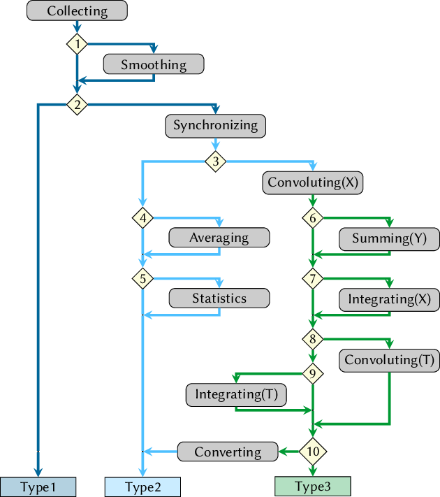
Possible workflows in data_collector.py.
Grey boxes denote the different computational actions, yellow diamonds denote the different decisions which are queried in the input dialog, and the boxes at the denote the three different data set types (dark blue=Type1, light blue=Type2, green=Type3).
The different actions and data set types are explained in the text.
Smoothing
In this step, each trajectory is individually smoothed, using one of several smoothing kernels (Gaussian, Lorentzian, Log-normal, rectangular).
Smoothing does not change the size or format of the data set, each value is simply replaced by the corresponding smoothed value; hence, a new Type1 data set is obtained.
Smoothing is applied to each X and each Y column independently, but always with the same kernel.
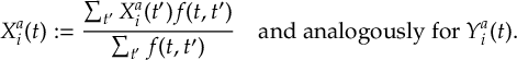
|
(7.1) |
Here, f(t,t′) is the smoothing kernel.
Synchronizing
In this step, the Type1 data set is reformatted, by merging all trajectories together.
This step creates a Type2 data set, which has a common T axis for all trajectories (simply the union of the T columns from all trajectories).
For each time step, all X and Y values of all trajectories are collected.
If a trajectories does not have data at a particular time step, NaNs will be inserted.
In this way, a rectangular, two-dimensional data set is obtained, with as many rows as time steps, and 2ntrajnX data columns.
A simple application of Collecting+Synchronizing could be to generate a table with the bond length for all time steps for all trajectories, in order to generate a “hair figure”.
This task could in principle also be accomplished with Bash tools like awk and paste, but this is troublesome if the trajectories are of different length, with different time steps, or if the table files contain comments.
Averaging
The Type2 data set from the Synchronizing step can contain a large number of data columns (2ntrajnX).
In order to reduce this amount of information, the Averaging step can be used to compute the mean and standard deviation across all trajectories, separately for each time step.
This will create a new Type2 data set, which still has a common time axis, but will only contain 4nX+1 data columns; these are the mean and standard deviation of all X and Y columns, plus one column giving the number of trajectories for each time step.
Currently, this step can be performed with either arithmetic mean/standard deviation or geometric mean/standard deviation.
Statistics
Similar to the Averaging step, the Statistics step computes mean and standard deviations from a Type2 data set.
The difference is that during Statistics, these values are computed for all values from the first to the current time step.
The data in the last time step thus gives the total statistics over all time steps and trajectories.
The Type2 data set from the Statistics step contains the same number of data columns as the one from the Averaging step.
Currently, this step can be performed with either arithmetic mean/standard deviation or geometric mean/standard deviation.
With the Averaging and Statistics steps, it is possible to compute the same data as with trajana_nma.py (if the appropriate files are read), namely the total (Statistics) and coherent (Averaging+Statistics) activity of the normal modes.
Using data_collector.py, the same analysis can also be applied to internal coordinates computed with geo.py.
Convoluting(X)
In order to create a data set which has common T and X axes (a Type3 data set), it is in general necessary to perform some kind of data convolution involving the X column data.
In order to do this, data_collector.py creates a grid along the X axis (ngrid points from the minimum value to the maximum value of all X data in the data set, plus some padding).
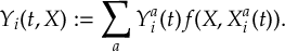
|
(7.2) |
The created Type3 data set has nX data points for each time step and each X grid point.
Using energies as X columns and oscillator strengths/intensities as Y columns, in this way it is possible to compute time-dependent spectra.
Summing(Y)
When nX is larger than one, the Summing step can be used to compute the sum over all data points for each time step and each X grid point.
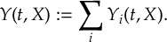
|
(7.3) |
This creates a new Type3 data set, which will only contain one data point for each time step and each X grid point.
For example, for a transient spectrum involving multiple final states (nX > 1), after the Convoluting(X) step one obtains one transient spectrum for each final state. With the Summing(Y) step, one can then compute the total transient absorption spectrum.
Integrating(X)
When computing transient spectra, one is often interested in integrating the spectrum within a certain energy window.
This can be done with the Integrating(X) step.
After entering a lower and upper X limit, a new Type3 data set is created, with only three data points per time step.
The first data point contains the integral from minus infinity to the lower limit, the second data point the integral between lower and upper limit, and the third data point the integral from the upper limit to infinity.
If Summing(Y) was not carried out, this integration is carried out independently for each of the nX data columns.
Convoluting(T)
The Type3 data set can also be convoluted along the time axis (e.g., in order to apply an instrument response function to a time-resolved spectrum).
In order to do this, a uniform grid along the T axis is generated (with nTgrid points from the minimum value to the maximum value of the previous T axis, plus some padding).
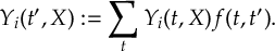
|
(7.4) |
The created Type3 data set has as many data points for each X grid point as before, but the number of time steps is now nTgrid.
Convoluting(T) can be applied also if Summing(Y) and/or Integrating(X) were used (in this case, the kernel is applied to the summed up or integrated data).
Integrating(T)
This step carries out a cumulative summation along the T axis.
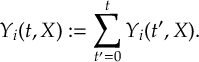
|
(7.5) |
In this way, the data in the last time step constitute the integral over all time steps.
Since all the partial cumulative sums are also computed, integrals within some bounds can simply be computed as differences between partial cumulative sums.
Converting
At the end of the workflow, a Type3 data set can be converted back into a Type2 data set, which affects how the output file is formatted.
This is usually a good idea if the Integrating(X) step was performed, but might not be a good idea otherwise.
See below for how the different data set types are formatted on output.
7.36.3 Output
After the input dialog is finished, data_collector.py will start carrying out the requested analyses.
For each of the workflow steps, one output file is written, so that all intermediate results can be used as well.
Output files have automatically generated filenames, which describe how the data was obtained.
Filenames are always in the form collected_data_<T>_<X>_<Y>_<steps>.<type>.txt, where <T> is an integer giving the T column index, <X> and <y> are lists of integers of the X and Y column indices, <steps> is a string denoting which workflow steps were carried out, and <type> denotes the data set type.
For example, an output file could be named collected_data_1_2_0_sy_cX.type3.txt, where column 1 was the T column, column 2 the X column, no Y column was used, Synchronizing and Convoluting(X) were performed, resulting in a Type3 data set.
Format of Type1 data set output
Type1 data sets are formatted such that each trajectory is given as a continuous block, separated by an empty line.
Within each block, each line contains the data of one time step, order increasingly.
Each line contains a trajectory index, the relative file path, the time, all X column data, and then all Y column data.
#    1                               2               3               4               5               6               7
#Index                        Filename            Time    X Column   5    X Column   6    Y Column   0    Y Column   0
     0 Singlet_1//TRAJ_00001/./Geo.out  0.00000000E+00  1.13340000E-01  7.99096900E+00  1.00000000E+00  1.00000000E+00
     0 Singlet_1//TRAJ_00001/./Geo.out  5.00000000E-01  1.59173000E-01  7.94395200E+00  1.00000000E+00  1.00000000E+00
     0 Singlet_1//TRAJ_00001/./Geo.out  1.00000000E+00  2.10868000E-01  7.89084000E+00  1.00000000E+00  1.00000000E+00
     ...
     1 Singlet_1//TRAJ_00002/./Geo.out  0.00000000E+00  5.03990000E-02  7.99078100E+00  1.00000000E+00  1.00000000E+00
     1 Singlet_1//TRAJ_00002/./Geo.out  1.00000000E+00  3.80370000E-02  8.00349700E+00  1.00000000E+00  1.00000000E+00
     1 Singlet_1//TRAJ_00002/./Geo.out  2.00000000E+00  1.09515000E-01  7.93073500E+00  1.00000000E+00  1.00000000E+00
     ...
     2 Singlet_1//TRAJ_00004/./Geo.out  0.00000000E+00  2.10908000E-01  8.29417600E+00  1.00000000E+00  1.00000000E+00
     2 Singlet_1//TRAJ_00004/./Geo.out  5.00000000E-01  1.49506000E-01  8.35651800E+00  1.00000000E+00  1.00000000E+00
     2 Singlet_1//TRAJ_00004/./Geo.out  1.00000000E+00  1.05887000E-01  8.40056700E+00  1.00000000E+00  1.00000000E+00
     ...
Note here in the example that the second trajectory has a time step of 1.0 fs and thus no data at 0.5 fs.
Format of Type2 data set output
Type2 data sets are formatted such that all trajectories share a common time axis, hence for each time step there will be one line of data.
Each line starts with the time, followed columns with the data for the first trajectory, followed by the data for the second trajectory, etc.
Within each trajectory, first all X columns, then all Y columns are given. If a Y column contains only unit weights (using special file column “0”), then this Y column is omitted from the Type2 formatted output.
#             1               2               3               4               5               6               7  ...
#          Time    X Column   5    X Column   6    X Column   5    X Column   6    X Column   5    X Column   6  ...
 0.00000000E+00  1.13340000E-01  7.99096900E+00  5.03990000E-02  7.99078100E+00  2.10908000E-01  8.29417600E+00  ...
 5.00000000E-01  1.59173000E-01  7.94395200E+00             NaN             NaN  1.49506000E-01  8.35651800E+00  ...
 1.00000000E+00  2.10868000E-01  7.89084000E+00  3.80370000E-02  8.00349700E+00  1.05887000E-01  8.40056700E+00  ...
 ...
Note here in the example that the second trajectory does not have data at 0.5 fs.
Format of Typ3 data set output
Type3 data sets are formatted such that all trajectories share common time and X axes.
The data is formatted block-wise, with the first block corresponding to the first time step and containing all points on the X grid, followed by an empty line, followed by the second block, etc.
Each block consists of ngrid lines, each starting with the time and X value in the first two columns and followed by nX columns with the convoluted data.
#             1               2               3               4
#          Time          X_axis       Conv(5,0)       Conv(6,0)
 0.00000000E+00 -1.45534000E-01  2.38544715E-05  0.00000000E+00
 0.00000000E+00  2.30671958E-01  1.51462322E+00  0.00000000E+00
 0.00000000E+00  6.06877917E-01  1.07930050E-01  0.00000000E+00
 ...
 5.00000000E-01 -1.45534000E-01  1.31312692E-04  0.00000000E+00
 5.00000000E-01  2.30671958E-01  1.28614756E+00  0.00000000E+00
 5.00000000E-01  6.06877917E-01  4.46251462E-10  0.00000000E+00
 ...
 1.00000000E+00 -1.45534000E-01  8.75871124E-05  0.00000000E+00
 1.00000000E+00  2.30671958E-01  2.42291042E+00  0.00000000E+00
 1.00000000E+00  6.06877917E-01  1.60277894E-16  0.00000000E+00
 ...
7.37 Delay time distributions: delay_time.py
This script performs an event time analysis and computes delay times between two independent events in each trajectory.
Here, an event is taken as a moment in time in which a certain variable of a trajectory crosses a given threshold for the first time.
For example, one could monitor a bond length and define the event as the first time that this bond length is larger than 3.5 Å.
Now one could define a second event as the first time that the active electronic state is lower than the S2.
With these two events defined, one could then compute the delay between the moment where the S1 state is entered and the bond becomes longer than 3.5 Å.
This delay could then be used to describe the time it takes the molecule to dissociate once the dissociative state is entered.
In practice, the script requires for each trajectory included in the analysis two files (although one could use the same file twice).
Each file should contain time-resolved data, with at least two columns (time and some variable).
The script produces a list of events and their time delay, as well as a histogram.
7.37.1 Usage
delay_time.py is an interactive script, which is started with:
user@host> $SHARC/delay_time.py
7.37.2 Input
Paths to trajectories
This part works just as in other interactive scripts.
The script asks the user to specify all directories for whose content the analysis should be performed. Enter one directory path at a time, and finish the directory input section by typing “end“. Please do not specify each trajectory directory separately, but specify their parent directories, e.g. the directories Singlet_1 and Singlet_2. crossing.py will automatically include all trajectories contained in these directories.
If you want to exclude certain trajectories from the analysis, it is sufficient to create an empty file called CRASHED or RUNNING in the corresponding trajectory directory. crossing.py will ignore all directories containing one of these files.
Additionally, align_and_reorder_traj.py will ignore trajectories with a DONT_ANALYZE file from diagnostics.py.
Note that this script cannot provide any hard evidence for causality, only for correlation of events in time.
Data files and columns
After all trajectories are included, the script provides a list of common files (similar to data_collector.py).
The user should then select the two files.
The order of the files is arbitrary but affects the sign of the delay distribution.
It is recommended to select as File 1 the file whose event is expected to happen first.
After selecting the two file paths (within each trajectory), next the user needs to provide the column indices for the time column and the data column in each file.
After selecting the file paths and time and data columns, effectively one obtains two data time series X1i(t) and X2i(t) for trajectory i.
Event thresholds
Then, the user needs to specify a threshold for each of the two data sets X1(t) and X2(t).
The threshold has to be given in whatever unit X1(t) and X2(t) are provided in the files.
Event detection method
The last input selects the event detection method.
Currently, two detection methods are implemented.
With the “simple” method, for each trajectory the first set is scanned for a point where X1(t) < T1 < X1(t+∆t) or X1(t) > T1 > X1(t+∆t).
If such a time t is found, the event is registered at time t1=t+[(∆t)/2].
Then the process is repeated with the X2 data, giving event time t2.
Then the delay is computed as t1−t2 for that trajectory.
With the “persistence” method, a tentative threshold crossing is first identified in the same way as for the simple method.
However, instead of immediately registering an event, the algorithm checks whether the signal remains on the new side of the threshold for at least a user-defined persistence time.
For an upward crossing, this means that X(t) ≥ T must hold continuously after the crossing; for a downward crossing, X(t) ≤ T must hold.
If the signal recrosses the threshold before the persistence time has elapsed, the candidate event is discarded.
Only if the condition is satisfied for the full persistence interval is the event confirmed, and the event time is assigned as t1=t+[(∆t)/2], corresponding to the initial crossing.
The same procedure is then applied to the X2 data to obtain t2, and the delay is computed as t1−t2 for that trajectory.
7.37.3 Output
The script produces the two files delay_times.out and delay_histogram.out.
The file delay_times.out is a text file with 8 columns:
- Trajectory i (continuously indexed, not using the initconds/trajectory indices),
- Registered event time t1 in fs (nan if no event was found),
- Registered event time t2 in fs (nan if no event was found),
- Time delay ∆t in fs,
- The direction of crossing for the event at t1: 1 for a crossing from below to above, and -1 for a crossing from above to below,
- The direction of crossing for the event at t2,
- The path to the first file,
- The path to the second file.
The file delay_histogram.out is another text file, with the following format:
     -3.56 -       1.00 fs: 134
      1.00 -       5.56 fs: 17
      5.56 -      10.12 fs: 303
     10.12 -      14.69 fs: 64
     14.69 -      19.25 fs: 116
The histogram bins are automatically assigned with the Freedman-Diaconis rule.
If the user prefers another binning scheme, we recommend to load the individual delay times from delay_times.out and building a histogram manually.
7.38 Handling large sets of coordinate data: align_and_reorder_traj.py
The script align_and_reorder_traj.py can be used to do two tasks simultaneously-(i) aligning the coordinate (and velocities) of trajectories and (ii) storing the coordinates resorted, with one file per time step instead of one file per trajectory.
This script reads one NetCDF file with coordinates (and velocities) from each trajectory; it either reads output.dat.nc or output_NUC.dat.nc.
Using the Kabsch algorithm, it translates and rotates a selected part of the system onto a reference geometry.
It then stores one file per time step, containing the coordinates from all trajectories for that time step.
The output is also using NetCDF files, but these NetCDF files are compliant with the format used by AMBER.
Hence, the resulting files can be read by VMD and cpptraj for further analysis.
7.38.1 Usage
align_and_reorder_traj.py is an interactive script, which is started with:
user@host> $SHARC/align_and_reorder_traj.py
7.38.2 Input
Paths to trajectories
This part works just as in other interactive scripts.
The script asks the user to specify all directories for whose content the analysis should be performed. Enter one directory path at a time, and finish the directory input section by typing “end“. Please do not specify each trajectory directory separately, but specify their parent directories, e.g. the directories Singlet_1 and Singlet_2. crossing.py will automatically include all trajectories contained in these directories.
If you want to exclude certain trajectories from the analysis, it is sufficient to create an empty file called CRASHED or RUNNING in the corresponding trajectory directory. crossing.py will ignore all directories containing one of these files.
Additionally, align_and_reorder_traj.py will ignore trajectories with a DONT_ANALYZE file from diagnostics.py.
Coordinate file
Here, the user get prompted to select either output.dat.nc or output_NUC.dat.nc.
The former is the default, the latter is only offered if such files are present.
Which file to use depends on whether you have used output_format netcdf or output_format netcdf_separate_nuclei in the SHARC input.
Reference geometry
Here you provide a file in xyz format with the reference geometry to which you want to align (part of) your system.
The atoms in the reference file should have the same ordering as in the SHARC trajectories.
Reference atom map
If you only want to align part of the system (e.g., the QM region of a QM/MM calculation), here you specify the atom numbers of the atoms that should be aligned.
This list must have the same length as the reference geometry has atoms.
If the reference geometry has a different atom ordering as the atoms in the SHARC trajectory, one can provide the indices in the correct way here; but this is error-prone and not recommended.
Perspective
Here one can choose between two options.
When using the “molecular perspective”, the molecule (i.e., the atoms in the reference atom map) is aligned optimally to the reference geometry at each individual time step.
This minimizes motion of the molecule, so that one can observe the distribution of solvent around the molecule.
This option removes self-rotation of the molecule, but because the frame of reference is different in each time step, this perspective is not an inertial frame.
Alternatively, one can use the “solvent perspective”.
Here, the translation and rotation operation is determined for each trajectory only from the first time step, and the same operations are then applied to later time steps.
This leads to a proper inertial frame of reference.
Here, one can observe that the molecule can rotate away from the reference orientation for later time steps, just as in reality.
Output files
Here one can choose to write or not write the coordinates and/or the velocities.
The default, and probably most used, option is to write only coordinates.
7.38.3 Output
The script creates, in the present directory, one NetCDF file per time step covered by the selected trajectories.
The files are called frame_coord_mol_pers_XXXXX.nc or frame_coord_sol_pers_XXXXX.nc, depending on the chosen perspective.
These files use all the settings needed to open them in VMD or cpptraj; note that you need a corresponding prmtop file in either case.
7.39 Producing radial distribution functions: frames_to_RDF.py
This script is used together with the output NetCDF files from align_and_reorder_traj.py (Section 7.38).
It calculates the radial distribution function (RDF) or radial histogram between two sets of atoms A and B over all snapshots t in the NetCDF file.
The histogram is defined as:
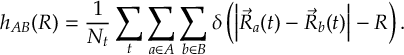
|
(7.6) |
The RDF is related to the histogram by
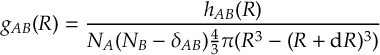
|
(7.7) |
where δAB=1 if the sets A and B are identical.
Hence, the RDF is a normalized version of the histogram, although the normalization of the RDF is missing the volume of the system and hence the RDF will not approach 1 at long distances, as it should.
We recommend to renormalize manually.
The script also computes the Cartesian-weighted histogram, which for the x component is
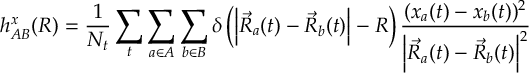
|
(7.8) |
and analogously for y and z.
Note that hAB(R)=hABx(R)+hABy(R)+hABz(R).
The same applies to the RDFs.
Note that this script tries to use numba for just-in-time compilation, if numba is installed.
This dramatically improves performance.
Note that the script caches the compiled code so that it can be reused when the script is called again.
However, this only works if all numerical parameters (especially the masks) are identical between the calls.
Hence, if operating on a large number of files, try to arrange your computations such that you loop over the NetCDF files in the innermost loop.
7.39.1 Usage
frames_to_RDF.py is a command-line, non-interactive script, which is started with:
user@host> $SHARC/frame_to_RDF.py <NetCDF> <mask1> <mask2> <outfile> [options]
7.39.2 Input
The script has four required input arguments.
The first argument is the path to the NetCDF file.
Note that NetCDF files that are produced by sharc.x or driver.py do not work, but files from align_and_reorder_traj.py (Section 7.38) do.
The second and third arguments are files specifying which atoms are in the sets A and B.
These files can be in either of two file formats: raw ASCII (one integer per line) or output files of cpptraj‘s mask command.
Note that these two files can be identical, but if they are not, they must not have shared indices (this limitation might get removed in the future).
The fourth argument is the desired output file name.
7.39.3 Options
The optional arguments are summarized in Table 7.19.
| Option | Description | Default |
| -h | Display help message and quit. | – |
| -w FLOAT | Bin width in Å | 0.1 |
| -n INT | Number of bins | 100 |
| -r | Write raw histograms | write RDFs |
7.39.4 Output
The output is an ASCII file with five columns.
The first column is the distance in Å, the second one is the histogram or RDF, and the three remaining columns are the x, y, and z component of the histogram or RDF.
7.39.5 Obtaining mask files
Mask files can be written manually.
They are simply an ASCII file with one integer per line, listing all the atoms that this mask encompasses.
Counting starts at 1.
Note that indices must not be repeated.
Alternatively, mask files can be written with cpptraj.
This requires a prmtop file and the NetCDF file that should be analyzed.
One starts cpptraj, loads the prmtop file, then the first frame of the NetCDF file, then uses the mask command to select some atoms (using AMBER‘s atom selection syntax), then runs the program:
[commandchars={}]
parm system.prmtop
trajin frame_coord_mol_pers_00000.nc 1 1
mask @mask @mask @mask @mask @run
quit
This produces a file that starts with Frame AtomNum Atom ResNum Res MolNum.
If this line is present, frames_to_RDF.py recognizes the format and reads the atom indices from the second column.
7.40 Producing 3D distributions: frames_to_dx.py
This script is used together with the output NetCDF files from align_and_reorder_traj.py (Section 7.38).
It calculates the three-dimensional distribution of atoms from a set A on a grid, using kernel density estimation.
Note that this script tries to use numba for just-in-time compilation, if numba is installed.
This dramatically improves performance.
The compiled code is not cached, unlike for frames_to_RDF.py.
7.40.1 Usage
frames_to_dx.py is a command-line, non-interactive script, which is started with:
user@host> $SHARC/frame_to_dx.py <NetCDF> <mask> <outfile> [options]
7.40.2 Input
The script has three required input arguments.
The first argument is the path to the NetCDF file.
Note that NetCDF files that are produced by sharc.x or driver.py do not work, but files from align_and_reorder_traj.py (Section 7.38) do.
The second argument is a file specifying which atoms are in the set A.
This file can be in either of two file formats: raw ASCII (one integer per line) or output files of cpptraj‘s mask command.
The mask files can be created as defined in Section 7.39.5.
The third argument is the desired output file name.
7.40.3 Options
The optional arguments are summarized in Table 7.20.
| Option | Description | Default |
| -h | Display help message and quit. | – |
| -w FLOAT | Cell width in Å | 0.5 |
| -n INT | Number of cells per direction | 40 |
| -f FLOAT | FWHM of the convolution Gaussian in Å | 0.5 |
| -c X,Y,Z | Center of the grid | origin |
7.40.4 Output
The output is an ASCII file containing grid data in OpenDX format.
The file specifies the position of the grid and the values of each grid cell.
These files can be visualized with VMD using the Isosurface representation.
See Ref. [37] for a discussion how to choose the isovalues needed for the Isosurface plots.
7.41 Computing X-ray scattering: RDF_to_scattering.py
This script takes the output of frames_to_RDF.py with the -r option and computes X-ray scattering using the independent atom model.
Note that the script is rather preliminary and has only limited options.
The data to compute the atomic form factors are taken from https://lampz.tugraz.at/~hadley/ss1/crystaldiffraction/atomicformfactors/formfactors.php, which employs linear combinations of Gaussian functions to model fi(Q).
The full function is:
|
(7.9) |
These atomic form factors can be used up until Q=25Å−1.
The scattering signal is computed as:

|
(7.10) |
Note that the script does not currently perform any smoothing or normalization.
Therefore, only difference scattering signals should be computed and no absolute intensities are obtained.
7.41.1 Usage
RDF_to_scattering.py is a command-line, non-interactive script, which is started like this (do not type the line break):
user@host> $SHARC/RDF_to_scattering.py --alpha <element1> --beta <element2>
           --hist <histogram> --hist-ref <reference> [options]
7.41.2 Input
The script requires several input arguments.
The -alpha and -beta flags specify the two elements for which the structure factor S(Q) is calculated.
These must match keys in the atomic form factor data file (e.g. h, o, li1+).
The keys are case-insensitive.
The -hist and -hist-ref flags give the paths to the files containing the pair distribution functions Hαβ(r) and Hαβref(r), respectively.
These files must contain at least two columns: the distance in Å in the first column and the histogram values in the user-selected column.
The form factor data file is specified with -data.
If SHARC is properly installed and the environment variable $SHARC is set, the default form factor file is taken from $SHARC/../lib/formfactor_gaussian.txt.
If this file exists, -data is optional, else it is required.
7.41.3 Options
The optional arguments are summarized in Table 7.21.
| Option | Description | Default |
| -data FILE | Form factor data file | $SHARC/../lib/formfactor_gaussian.txt |
| -alpha STR | Element α key | required |
| -beta STR | Element β key | required |
| -hist FILE | Histogram Hαβ(r) file | required |
| -hist-ref FILE | Reference histogram Hαβref(r) file | required |
| -column INT | Histogram column index (1-based) | 2 |
| -rcut FLOAT | Cutoff for maximum r (Å) | 10.0 |
| -qmax FLOAT | Maximum Q value (Å−1) | 15.0 |
| -qpoints INT | Number of Q points to compute | 200 |
| -h | Display help message and quit | – |
7.41.4 Output
The output is written to standard output and consists of two columns: the Q value and the corresponding structure factor S(Q).
Each line corresponds to a different Q value, spaced linearly between 0.01 and qmax with a total of qpoints values.
These results can be redirected into a file for plotting or further analysis:
user@host> ./RDF_to_scattering.py ... > sq.dat
7.42 Merging per-time-step-data: data_merger.py
When investigating RDFs or scattering results, one usually produces one RDF/scattering curve for each simulation time step.
This results in a large number of files that are awkward to print.
data_merger.py can merge these files into one large file for easier or 3D printing.
The script can additionally perform a temporal convolution on the data to mimic the temporal resolution of an experiment.
7.42.1 Usage
data_merger.py is a command-line, non-interactive script, which is started like this (do not type the line break):
user@host> $SHARC/data_merger.py <file_pattern> --output <outfile> [options]
7.42.2 Input
The script requires several input arguments.
First, the script requires one positional argument, the file pattern to read the RDF/scattering curves.
Other data, where each file contains at least two columns (e.g., a position and a value) and all files have the same length and position column, is also permissible.
The file names usually contain a number, e.g., RDF_000001.out, RDF_00001.out, …, and the files must reside in the present directory.
The file pattern for these example file names would be RDF_%05i.out.
Additionally, the script requires the -output option, where an output file name needs to be given.
7.42.3 Options
The optional arguments are summarized in Table 7.22.
| Option | Description | Default |
| -output STR | Output file name | required |
| -x-col INT | Column index for the x values (1-based) | 1 |
| -y-col INT | Column index for the y values (1-based) | 2 |
| -ref_av_n INT | Average the first N files to obtain the reference data | 1 |
| -time-step FLOAT | Time step (in fs) between files | 1 fs |
| -input-file STR | Path to an input file of a trajectory, to read time step and output stride | fixed 1 fs steps |
| -convolution INT | Choose convolution kernel (1: Gaussian, 2: Lorentzian, 3: Box, 4: Lognormal) | no convolution |
| -fwhm FLOAT | FWHM for the convolution kernel | required if convolution |
| -tmin FLOAT | Minimum time for convolution grid | required if convolution |
| -tmax FLOAT | Maximum time for convolution grid | required if convolution |
| -tpoints INT | Number of convolution grid points | required if convolution |
| -h | Display help message and quit | – |
7.42.4 Output
The output is written to the file indicated with -output.
It contains four columns: The time, the position (or whatever x data was provided), the values (y data), and the reference y values (average of the first -ref_av_n files).
If convolution is used, the time points do not necessarily agree with the times corresponding to each file.
Instead, they are given as an equally spaced temporal grid as defined by the corresponding options.
7.43 Optimizations: otool_external and setup_orca_opt.py
All SHARC interfaces can deliver gradients for (multiple) ground and excited states in a uniform manner.
This allows in principle to perform optimizations of excited-state minima, conical intersections, or crossing points.
In order to employ a high-quality geometry optimizer for this task, the SHARC suite is interfaced to the external optimizer feature of ORCA.
This is accomplished by providing the scripts orca_External (for ORCA4, will be deprecated in the near future) and otool_external (for ORCA5/6), which is called by ORCA, runs any of the SHARC interfaces, constructs the appropriate gradient, and returns that to ORCA.
For the methodology used to construct the gradients, see Section 8.20.
In order to easily prepare the input files for such an optimization, the script setup_orca_opt.py can be used.
It takes a geometry file, interface input files, and the path to ORCA, and creates a directory containing all relevant input files.
In the following, setup_orca_opt.py is described first, because it is the script which the user directly employs.
Afterwards, orca_External and otool_external are specified.
7.43.1 Usage
setup_orca_opt.py is an interactive script, which is started with:
user@host> $SHARC/setup_orca_opt.py
Note that before executing the script you should prepare a template for the interface you want to use (as, e.g., in setup_init.py or setup_traj.py).
7.43.2 Input
In the input section, the script asks for: (i) the path to ORCA, (ii) the input geometries, (iii) the optimization settings, (iv) the interface settings.
Path to ORCA
Here the user is prompted to provide the path to the ORCA directory. Note that the script will not expand the user ( ) and shell variables (since possibly the calculations are running on a different machine than the one used for setup). and shell variables will only be expanded during the actual calculation.
The script works with ORCA 4, 5, and 6.
Interface
In this point, choose any of the displayed interfaces to carry out the ab initio calculations.
Enter the corresponding number.
If you selected SHARC_LEGACY.py, then you have to subsequently select the legacy interface that you intend to use.
If you selected a hybrid interface, then you will subsequently be queried with the path to the corresponding template file, so that the hybrid interface can figure out the child interface it should use.
This might continue recursively until all interfaces in the interface call tree are known.
Input geometry
Here the user is prompted for a geometry file in XYZ format, containing one or more geometries (with consistent number of atoms).
For each geometry in this file, a directory with all input files is created, in order to carry out multiple optimizations (e.g., with output from crossing.py).
Number of states
Here the user can specify the number of excited states to be calculated. Note that the ground state has to be counted as well, e.g., if 4 singlet states are specified, the calculation will involve the S0, S1, S2 and S3. Also states of higher multiplicity can be given, e.g. triplet or quintet states.
Charge
As in other setup scripts, you need to provide the charge for each involved multiplicity.
States to optimize
Two different optimization tasks can be carried out: optimization of a minimum (ground or excited state) or optimization of a crossing point (either a conical intersection between states of the same multiplicity or a minimum-energy crossing points between states of different multiplicities; this is detected automatically).
For minima, the state to optimize needs to be specified.
For crossing points, the two involved states need to be specified.
In all cases, the specified states need to be included in the number of states given before.
CI optimization parameters
If you are optimizing a conical intersection (states of same multiplicity) with an interface which cannot provide nonadiabatic coupling vectors (e.g., SHARC_TURBOMOLE.py, SHARC_ADF.py, or SHARC_GAUSSIAN.py), then the optimization will employ the the penalty function method of Levine, Coe, and Martínez [73].
In this method, a penalty function is optimized, which depends on the energies of the two states and on two parameters, σ and α (see section 8.20 for their mathematical meaning).
Practically, the parameters affect how close the minimum of the penalty function is to the true minimum on the crossing seam and how hard the optimization will be to converge.
Generally, a large σ will allow going closer to the true conical intersection, but will make the penalty function more stiff (steeper harmonic) and thus harder to optimize.
A small α will also allow going closer to the true conical intersection, but will make the penalty function less harmonic; at α = 0, the penalty function will have a cusp at the minimum, making it unoptimizable because the gradient never becomes zero.
The default values, 3.5 and 0.02, are the ones suggested in [73].
They can be regarded as relatively soft, i.e., they enable a very smooth convergence but might lead to unacceptably large energy gaps at convergence (i.e., the minimum of the penalty function is too far from the true minimum of the crossing seam).
In this case, it is advisable to restart the optimization from the last point with increased σ (e.g., by a factor of 4), and simultaneously reducing the maximum step (see next point).
The α is best left at the suggested value of 0.02 to avoid the cusp problem.
For interfaces that can deliver nonadiabatic coupling vectors, instead the gradient projection technique of Bearpark et al.[72] is used.
For all interfaces, a similar projection method is used when optimizing intra-multiplicity crossings (e.g., singlet-triplet crossings), as no nonadiabatic coupling vectors are needed there.
Maximum allowed displacement
Within ORCA, it is possible to restrict the maximum step (the trust radius) of the optimizer.
A larger maximum step might decrease the number of iterations necessary, but might also lead to instabilities in the optimization (if the potential energy surface is very steep or anharmonic).
Hence, it can be advisable to reduce the maximum allowed step (from the default of 0.3 a.u.), especially if the starting geometry is already very good (e.g., after restart with increase of σ) or if the potential is known to be stiff (strong bond, large σ, small α, …).
Note that the maximum step can be restricted even the penalty function method is not used and σ and α are not relevant.
Interface-specific input
This input section is basically the same as for other setup scripts.
Note that for hybrid interfaces, all child interfaces will also ask for relevant input.
Run script setup
Here the user needs to provide the path to the directory where the optimizations should be setup.
7.43.3 Output
Inside the specified directory, setup_orca_opt.py creates one subdirectory for each geometry in the input geometry file.
Each subdirectory is prepared with the corresponding initial geometry file (geom.xyz), the ORCA input file (orca.inp), the file otool_external.inp, the appropriate interface-specific files, and a shell script for execution (run_EXTORCA.sh).
In order to run one of the optimizations, execute the shell script or send it to a batch queuing system.
Note that $SHARC needs to be added to the $PATH so that ORCA can find orca_External.
For ORCA6, the $EXTOPTEXE variable must be set.
(Both of these steps are automatically done inside run_EXTORCA.sh).
When the shell script is started, ORCA will write a couple of output files, where the two most relevant are orca_trj.xyz and orca.log.
The former is an XYZ file with all geometries from the optimization steps.
The latter (the ORCA standard output) contains all details of the optimization (convergence, step size, etc) as well as a summary of what orca_External did (after the line EXTERNAL SHARC JOB).
This summary contains all relevant energies and shows how the gradient is constructed.
Note that in each iteration, a line starting with >>> is written, which contains the energies of the optimized state(s). This line can easily be extracted with grep to follow the optimization of a crossing point.
For ORCA 6, this output is instead written to otool_external_all_output.txt.
7.43.4 Description of orca_External and otool_external
orca_External and otool_external provide a connection between the external optimizer of ORCA and any of the SHARC interfaces.
In figure 7.5, the file communication between ORCA, orca_External, and the interfaces is presented.
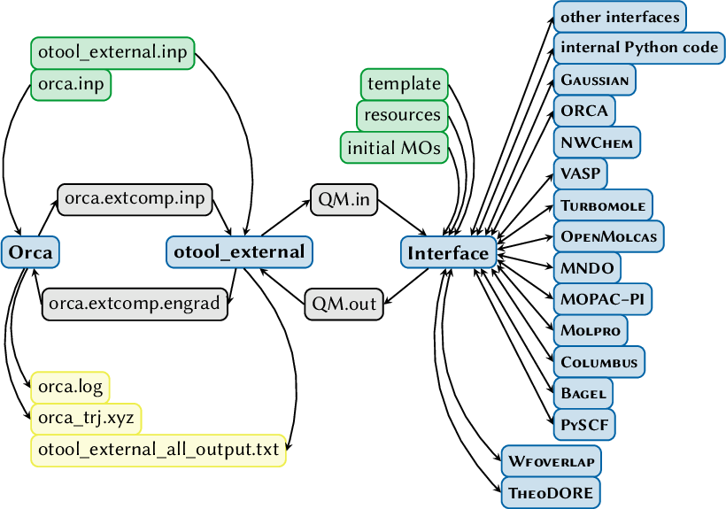
As can be seen, otool_external (or orca_External) writes QM.in and QM.out files, in the same way that sharc.x is doing.
All information to write the QM.in file comes from the ORCA communication file orca.extcomp.inp (geometry) and the ORCA input file (number of states, interface, states to optimize).
To provide the latter information, orca_External reads specially marked comments from the ORCA input file which are ignored by ORCA.
These comments start with #SHARC:, followed by a keyword (states, interface, opt, or param) and the keyword arguments.
When using otool_external, the settings are not read from orca.inp, because otool_external cannot work out the path to orca.inp in a robust way.
Instead, the settings are read from a separate file otool_external.inp that is created by setup_orca_opt.py.
Options inside otool_external.inp
The content of this file looks like this:
#SHARC: states 3 0 4
#SHARC: charge 1 0 1
#SHARC: opt [min|cross] <state> [<state2>]
#SHARC: interface <SHARC_INTERFACENAME>
#SHARC: params <sigma> <alpha>
These are parsed like this:
- states: This is interpreted like in any other part of SHARC. The numbers are verbatim transferred to the generated QM.in file and then read by the interface.
- charge: Like states, these numbers are verbatim transferred to the generated QM.in file and then read by the interface.
- opt This keyword is followed by either min or cross. The first selects a minimum (ground or excited state), the second a crossing point (minimum-energy conical intersection or minimum-energy crossing point, determined automatically). min is followed by 1 integer, the index of the state to optimize; cross is followed by 2 integers, the indices of the two states whose crossing is optimized (both options use state indices as in Section 8.28).
- interface: Selects the interface to use. It is acceptable to use either SHARC_XXX or simply XXX (e.g., both SHARC_LVC and LVC are allowed strings in this line).
- params: Followed by two floats that define σ and α as described above in Section 7.43.2.
7.44 Single Point Calculations: setup_single_point.py
It is possible to run single point calculations through the SHARC interfaces.
This is useful, e.g., to do a computation in exactly the same way as during the dynamics simulations.
Single point calculations using the interfaces can also be easily automatized.
7.44.1 Usage
setup_single_point.py is an interactive script, which is started with:
user@host> $SHARC/setup_single_point.py
Note that before executing the script you should prepare a template for the interface you want to use (as, e.g., in setup_init.py or setup_traj.py).
7.44.2 Input
In the input section, the script asks for: (i) the input geometries, (ii) the number of states, and (iii) the interface settings.
Interface
In this point, choose any of the displayed interfaces to carry out the ab initio calculations.
Enter the corresponding number.
If you selected SHARC_LEGACY.py, then you have to subsequently select the legacy interface that you intend to use.
If you selected a hybrid interface, then you will subsequently be queried with the path to the corresponding template file, so that the hybrid interface can figure out the child interface it should use.
This might continue recursively until all interfaces in the interface call tree are known.
Input geometry
Here the user is prompted for a geometry file in XYZ format, containing one or more geometries (with consistent number of atoms).
For each geometry in this file, a directory with all input files is created, in order to carry out multiple optimizations (e.g., with output from crossing.py).
Number of states
Here the user can specify the number of excited states to be calculated. Note that the ground state has to be counted as well, e.g., if 4 singlet states are specified, the calculation will involve the S0, S1, S2 and S3. Also states of higher multiplicity can be given, e.g. triplet or quintet states.
Charge
As in other setup scripts, you need to provide the charge for each involved multiplicity.
Interface-specific input
This input section is basically the same as for other setup scripts.
Note that for hybrid interfaces, all child interfaces will also ask for relevant input.
Run script setup
Here the user needs to provide the path to the directory where the optimizations should be setup.
7.44.3 Output
Inside the specified directory, setup_single_point.py creates one subdirectory for each geometry in the input geometry file.
Each subdirectory is prepared with the corresponding geometry file (QM.in), the appropriate interface-specific files (template, resources, QM/MM), and a shell script for execution (run.sh).
In order to run one of the optimizations, execute the shell script or send it to a batch queuing system.
When the shell script is started, the chosen SHARC interface is executed.
The interface writes a file called QM.log which contains details of the computation and progress status.
The final results of the computation are written to QM.out, which can be inspected manually.
Alternatively, some basic data (excitation energies, oscillator strengths) can be computed with QMout_print.py (section 7.45).
7.45 Format Data from QM.out Files: QMout_print.py
With the script QMout_print.py one can print a table with energies and oscillator strengths from a QM.out file, as it is produced by the interfaces.
7.45.1 Usage
QMout_print.py is a command line tool, and is executed like this:
user@host> $SHARC/QMout_print.py [options] QM.out
The options are summarized in Table 7.23.
Note that from SHARC 4.1, it is not necessary anymore to give the number of states with the -s option.
| Option | Description | Default |
| -h | Display help message and quit. | – |
| -e FLOAT | Absolute energy shift in Hartree | 0.0 |
| -D | Output diagonal states | MCH states |
| -S STATE | Initial state index | 1 |
| -L | Format output in a single line (useful for scans) | false |
| -I | Use Dyson norms instead of oscillator strengths | false |
7.45.2 Output
The script prints a table with state index, state label, energy, relative energy, oscillator strength, and spin expectation value to standard output.
Chapter 8 Methods and Algorithms
In this chapter different aspects of SHARC simulations are discussed in detail. The topics are ordered alphabetically.
8.1 Absorption Spectrum
Using spectrum.py, an absorption spectrum can be calculated as the sum over the absorption spectra of each individual initial condition:
|
(8.1) |
where i runs over the initial conditions.
The spectrum of a single initial condition is the convolution of its line spectrum, defined through a set of tuples (Eα,foscα) for each electronic state α, where Eα is the excitation energy and foscα) is the oscillator strength.
The convolution of the line spectrum can be performed with spectrum.py using either Gaussian or Lorentzian functions. The contribution of a state α to the absorption spectrum σα(E) is given by:
|
(8.2) |
|
(8.3) |
or
|
(8.4) |
|
(8.5) |
or
|
(8.6) |
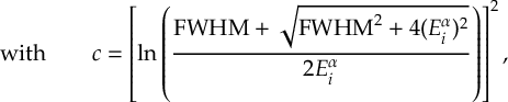
|
(8.7) |
where FWHM is the full width at half maximum.
8.2 Active and inactive states
SHARC allows to “freeze” certain states, which then do not participate in the dynamics. Only energies and dipole moments are calculated, but all couplings are disabled. In this way, these states are never visited (hence also no gradients and nonadiabatic couplings are calculated, making the inclusion of these states cheap). Example:
nstates 2 0 2
actstates 2 0 1
In the example given, state T2 is frozen. The corresponding Hamiltonian looks like:
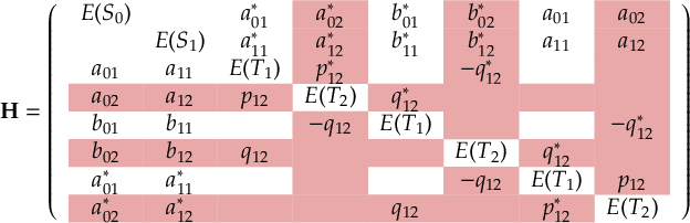
|
(8.8) |
where all matrix elements marked
| red |
are deleted, since T2 is frozen.
The corresponding matrix elements are also deleted from the nonadiabatic coupling and overlap matrices. For propagation including laser fields, also the corresponding transition dipole moments are neglected, while the transition dipole moments still show up in the output (in order to characterize the frozen states).
Active and frozen states are defined with the states and actstates keywords in the input file. Note that only the highest states in each multiplicity can be frozen, i.e., it is not possible to freeze the T1 while having T2 active. However, it is possible to freeze all states of a certain multiplicity.
8.3 Amdahl’s Law
Some of the interfaces (SHARC_MOLCAS.py, SHARC_ADF.py SHARC_GAUSSIAN.py, SHARC_ORCA.py) use Amdahl’s law to predict the most efficient way to run multiple calculations in parallel, where each calculation itself is parallelized.
For example, in SHARC_GAUSSIAN.py it might be necessary to compute the gradients of five states, using four CPU cores.
The most efficient way to run these five jobs depends on how well the GAUSSIAN computation scales with the number of cores-for bad scaling, running four jobs on one core each followed by the fifth job might be best, whereas for good scaling, running each job on four cores subsequently is better because no core is idle at any time.
In order to automatically distribute the jobs efficiently, the interfaces use Amdahl’s law, which can be stated as:
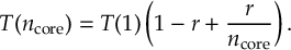
|
(8.9) |
Here, T(1) is the run time of the job with one CPU core, and r is the fraction of T(1) which benefits from parallelization.
The parameter r can be given to the interfaces; it is between 0 and 1, where 0 means that the calculation does not get faster at all with multiple cores, whereas 1 means that the run time scales linearly with the number of cores.
8.4 Bootstrapping for Population Fits
Bootstrapping, in the context of population fitting, is a statistical method to obtain the statistical distribution of the fitted parameters, which can be used to infer the error associated with the fitted parameter.
The general idea of bootstrapping is to take the original sample (the set of trajectories in the ensemble), and generate new samples (resamples) by randomly drawing trajectories “with replacement” from the original ensemble.
These resamples will differ form the original ensemble by containing some trajectories multiple times while other trajectories might be missing.
For each of the resamples, the fitting parameter are obtained normally and saved for later analysis.
After many resamples, we obtain a list of many “alternative” parameters, which can be plotted in a histogram to see the statistical distribution of the fitting parameter.
The number of resamples should generally be large (several hundred or thousand resamples), although with bootstrap.py, one can inspect the convergence of the fitting parameters/errors to decide how many resamples are sufficient.
From the computed list of parameters, error measures can be computed.
Assume that {xi} is the set of fitting parameters obtained.
bootstrap.py and make_fit.py compute the arithmetic mean and standard deviation like this:
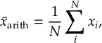
|
(8.10) |
|
(8.11) |
Because the distribution of {xi} might be skewed (e.g., contains some very large values but few very small ones), the script also computes the geometric mean and standard deviation like this:
|
(8.12) |
|
(8.13) |
Note that the geometric standard deviation is a dimensionless factor (unlike the arithmetic standard deviation, which has the same dimension as the mean).
Therefore, within bootstrap.py and make_fit.py the geometric errors are always displayed with separate upper and lower bounds as ―x\substack+―x(σ(x)−1) −―x(1/σ(x)−1).
Note that bootstrap.py and make_fit.py will always report one times the standard deviation in the output.
If larger confidence intervals are desired, simply multiply the arithmetic error as usual.
For the geometric error, use for example ―x\substack+―x(σ(x)2−1) −―x(1/σ(x)2−1).
8.5 Computing electronic populations
The electronic populations from SHARC trajectories can be obtained in different ways.
This is primarily due to the fact that in surface hopping one could either consider the active state or the electronic wave function coefficients.
This issue is discussed in detail in [77], where it is shown that the optimal way to obtain the electronic populations is actually a combination of both kinds of information in a Wigner-like transformation.
Hence, there are three options in SHARC: (i) based on classical active state, (ii) based on electronic wave function coefficients, and (iii) based on Wigner-transform.
Additionally, the populations can be analyzed in different representations (diagonal, MCH, diabatic).
Diagonal representation
The diagonal representation, there is no basis transformation involved, and hence the equations are very simple.
For a single trajectory, the three possible populations can be obtained by:
|
(8.14) |
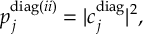
|
(8.15) |
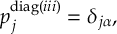
|
(8.16) |
where α is the active diagonal state.
MCH representation
To obtain the MCH representation, one needs to transform the populations with the matrix U.
Hence, one obtains:
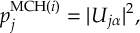
|
(8.17) |
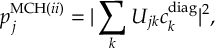
|
(8.18) |
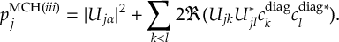
|
(8.19) |
Diabatic representation
To obtain the diabatic representation, one needs to transform the populations with the appropriate transformation matrix T, which in SHARC is obtained as the matrix product of reference overlap matrix, time-ordered overlap matrices, and U for the current time step.
Hence, one obtains:
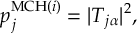
|
(8.20) |
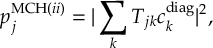
|
(8.21) |
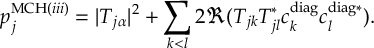
|
(8.22) |
8.6 Damping
If damping is activated in SHARC (keyword dampeddyn), in each time step the following modification to the velocity vector is made
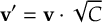
|
(8.23) |
where C is the damping factor given in the input. Hence, in each time step the kinetic energy is modified by
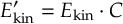
|
(8.24) |
The damping factor C must be between 0 and 1.
8.7 Decoherence
In surface hopping, without any corrections the coherence between the states is usually too large [21]. A trajectory in state β, but where state α has a large coefficient, will still travel according to the gradient of state β. However, the gradients of state α are almost certainly different to the ones of state β. As a consequence, too much population of state α is following the gradient of state β. Decoherence corrections damp in different ways the population of all states α ≠ β, so that only population of β follows the gradient of state β.
Currently, in SHARC there are two decoherence corrections implemented, “energy-based decoherence”, or EDC, as given in [108] and “augmented fewest-switches surface hopping”, or AFSSH, as described in [39].
8.7.1 Energy-based decoherence
In this scheme, after the surface hopping procedure, when the system is in state β, the coefficients are updated by the following relation
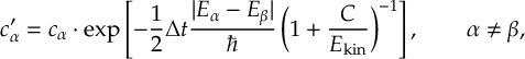
|
(8.25) |
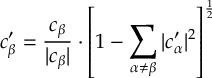
|
(8.26) |
where C is the decoherence parameter. The decoherence correction can be activated with the keyword decoherence in the input file. The decoherence parameter C can be set with the keyword decoherence_param (the default is 0.1 hartree, as suggested in [108]).
8.7.2 Augmented FSSH decoherence
Augmented FSSH by Subotnik and coworkers is described in [39].
For SHARC, the augmented FSSH algorithm was adjusted to the case of the diagonal representation.
The basic idea is that besides the actual trajectory, the program maintains an auxiliary trajectory for each state.
The auxiliary trajectories are propagated using the gradients of the associated (not active) state, and because the gradients are different, the auxiliary trajectories eventually diverge from each other and from the main trajectory.
From this diverging, one can compute decoherence rates which can be used to stochastically set the electronic coefficients of the diverging state to zero.
First, we compute two matrices:

|
(8.27) |

|
(8.28) |
where S is the overlap matrix, as used in 8.33.
Hence, Sdiag(t,t+∆t) is the overlap matrix in the diagonal basis and Holddiag(t+∆t) is the Hamiltonian at time t+∆t expressed in the diagonal basis of time step t.
We then propagate the auxiliary trajectories for each state j, considering that the active state is α.
For this, we need the gradient matrix Gdiag from section 8.11.
We define:
|
(8.29) |
We do the X step of the velocity-Verlet algorithm:
|
(8.30) |
|
(8.31) |
where A goes over the atoms.
Then, we compute the new gradient:
|
(8.32) |
We then carry out the v step:
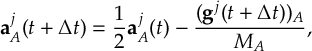
|
(8.33) |
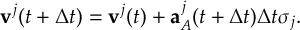
|
(8.34) |
We then perform a diabatization of the auxiliary trajectories (e.g., for a trivially avoided crossing, the moments between the crossing states are interchanged):
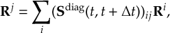
|
(8.35) |
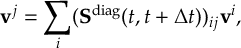
|
(8.36) |

|
(8.37) |
to transform the data back into the adiabatic basis at time t+∆t.
Finally, we carry out the decoherence correction procedure for each auxiliary trajectory.
We compute the displacement from the auxiliary trajectory of the active state:
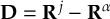
|
(8.38) |
We compute two rate constants:
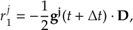
|
(8.39) |
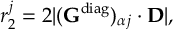
|
(8.40) |
or if no nonadiabatic coupling vectors are available:
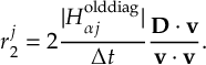
|
(8.41) |
We draw a random number (identical for all states) r between 0 and 1.
If r < ∆t(rj1−rj2), then we collapse state j, by setting its coefficient to zero and enlarging the coefficient of the active state such that the total norm is conserved; we also set the moments Rj and vj to zero.
If no collapse occurred, if r < −∆t rj1, we set the moments Rj and vj to zero.
After a surface hop occurred, we reset all auxiliary trajectories.
8.8 Essential Dynamics Analysis
As an alternative to normal mode analysis (see section 8.19), essential dynamics analysis can be used to identify important modes in the dynamics.
This procedure is a principal component analysis of the geometric displacements.[70,[69]
Unlike normal mode analysis, it does not depend on the availability of the normal mode vectors.
The covariance matrix is computed from the following equation (μ and ν are indices over the 3Natom degrees of freedom):
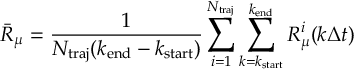
|
(8.42) |
and
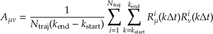
|
(8.43) |
as a matrix C with elements:
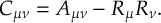
|
(8.44) |
Diagonalization of the symmetric matrix C gives a set of eigenvalues and eigenvectors.
The eigenvectors represent the essential dynamics modes, and the corresponding eigenvalues are the variances of the modes.
Modes with large variances show strong motion in the dynamics, whereas small variances are found for modes which show weak motion.
Because the modes are uncorrelated, the few modes with the largest variance describe most of the molecular motion, which shows that essential dynamics analysis can be used to for data reduction.
8.9 Excitation Selection
excite.py can select initial active states for the dynamics based on the excitation energies Ek,α and the oscillator strengths fosck,α for each initial condition k and excited state α.
First, for all excited states of all initial conditions, the maximum value pmax of
 |
(8.45) |
is found. Then for each excited state, a random number rk,α is picked from [0,1]. If

|
(8.46) |
then the excited state is selected as a valid initial condition. This excited-state selection scheme is taken from [125].
Within excite.py it is possible to restrict the selection to a subset of all excited states (only certain adiabatic states/within a given energy range). In this case, also pmax is only determined based on this subset of excited states.
8.9.1 Excitation Selection with Diabatization
The active states can be selected based on a diabatization.
This necessitates the wave function overlaps between a reference geometry (ICOND_00000/) and the current initial condition k.
The overlap matrix with elements
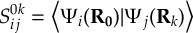
|
(8.47) |
can be computed with wfoverlap.x (calculations can be setup with setup_init.py).
This overlap matrix is rescaled during the excitation selection procedure such S0k11 is equal to one (by dividing all elements by |S0k11|2).
Then, assume we want to start all trajectories in the state which corresponds to state x at the reference geometry.
The excitation selection will select a state y as initial state if S0kxy > 0.5.
8.10 Global fits and kinetic models
In this section, we specify the basic assumptions of the chemical kinetic models used with the scripts make_fitscript.py and make_fit.py and the globals fits of these models to data.
8.10.1 Reaction networks
The kinetic models used by make_fitscript.py and make_fit.py are based on a chemical reaction network, where chemical species react via unimolecular reactions.
The reaction networks allowed in the script are a simple directed graphs, where the species are the vertices and the reactions are the directed edges.
Each reaction is characterized by an associated rate constant and connects exactly one reactant species to exactly one product species.
In order to obtain rate laws which can be integrated easily, there are a number of restrictions imposed on the network graphs.
Some restrictions and possible features of the graphs are depicted exemplarily in Figure 8.1.
First, each species and each reaction rate needs to have a unique label.
There cannot be two species with the same label, but there can be two reactions with the same reaction rate constant.
Second, the graph must be a simple directed graph, hence there cannot be any (self-) loops or more than one reaction with the same initial and the same final species.
All restrictions marked as “Not allowed” in the Figure are enforced in the input dialogue of make_fitscript.py
However, back reactions are allowed (as a back reaction has a different initial and a different final species as the corresponding reaction).
Except from these restrictions, the graph may contain combinations of sequential and parallel reactions.
The graph may also be disjoint, i.e., it can be the union of several independent sub-networks.
Disjoint graphs with repeated reaction labels can be useful to fit population data from ensembles with identical settings but different initial conditions (in this case, merge the population files with paste before starting the fit.
There are two kinds of cycles possible, called here parallel pathways and closed walks.
Parallel pathways are independent sequences of reactions with the same initial and final species (e.g., A→ C and A→ B→ C).
A closed walk is a sequence of reactions where the initial species is equal to the final species.
These cycles can sometimes lead to problems.
If you use make_fitscript.py, then it is necessary that the system of differential equations of the rate laws can be integrated in closed form by MAXIMA.
Since make_fit.py solves the differential equation system numerically, it is not necessary that the solution can be given in closed form.
However, cycles can also lead to problems in the fitting procedure (rate constants in parallel pathways can be strongly correlated and cause large errors and bad convergence in fitting).
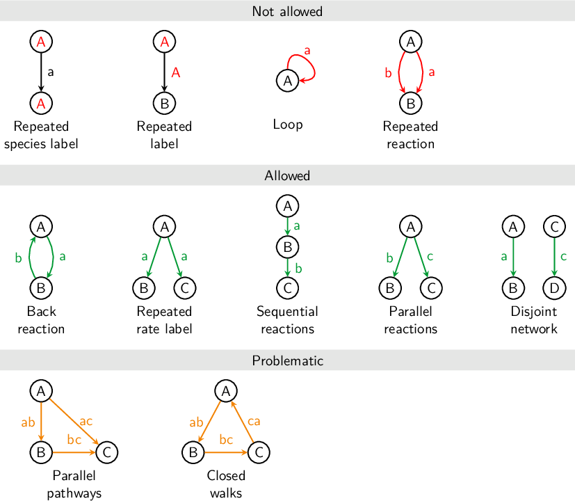
An example reaction network graph is shown in Figure 8.2.
In this graph, there are 5 species (S2, S1, S0, T2, and T1) and 6 reactions, each with a rate constant (kS, kRlx, k22, k11, k21, k12).
This graph shows some features which are allowed in the reaction networks for make_fitscript.py: sequential reactions, parallel reactions, back reactions, and converging reaction pathways.
Note that this reaction network is likely to cause problems in the fitting step (large errors).
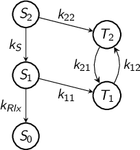
8.10.2 Kinetic models
Based on the reaction network graph, a system of differential equations describing the rate laws of all species can be setup.
The system of equations (equivalently, the matrix differential equation) can be written as:
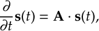 |
(8.48) |
where s is the vector of the time-dependent populations of each species and A is the matrix containing the rate constants.
In order to construct A, start with A=0 and, for each reaction from species i to species j with rate k, substract k from Aii and add k to Aji.
In order to integrate this system of equations, in practice one also needs to define initial conditions.
In the present context, the initial conditions are fully specified by s(t=0)=s0, where s0 are constant expressions defined by the user.
Solving (8.48) yields (in not too complicated cases) the closed-form expressions for the functions s(t), which contain as parameters all rate constants k and all initial values s0.
8.10.3 Global fit
Suppose there is a data set p(t)=(p1(t),p2(t),…) of time-dependent populations of several states k=1,2,… and which is given at several points of time {ti: 0 < ti < tmax}.
We can fit to one data set pk(t) a function sl(t) from s(t) by optimizing the parameters (mainly the rate constants) such that ∑i |pk(ti)−sl(ti)|2 becomes minimal.
In order to perform global fit including several species l and several states k, we construct piecewise global functions from p(t) and s(t) and then optimize the parameters accordingly.
8.11 Gradient transformation
8.11.1 Nuclear gradient tensor transformation scheme
Since the actual dynamics is performed on the PESs of the diagonal states, also the gradients have to be transformed to the diagonal representation. To this end, first a generalized gradient matrix GMCH is constructed from the gradients gMCHα=−∇RHααMCH
and the nonadiabatic coupling vectors
KβαMCH:
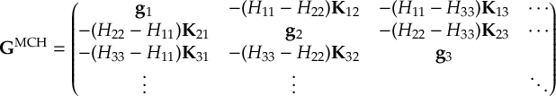
|
(8.49) |
Note that all quantities in the matrix are in the MCH representation, the superscripts were omitted for brevity.
The matrix GMCH is subsequently transformed into the diagonal representation, using the transformation matrix U:
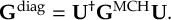
|
(8.50) |
The diagonal elements of Gdiag now contain the gradients of the diagonal states, while the off-diagonal elements contain the scaled nonadiabatic couplings −(Hdiagββ−Hdiagαα)Kβαdiag. The gradients are needed in the Velocity Verlet algorithm in order to propagate the nuclear coordinates. The nonadiabatic couplings are necessary if the velocity vector is to be rescaled along the nonadiabatic coupling vector.
Since the matrix GMCH contains elements which are itself vectors with 3N components, the transformation is done component-wise (e.g. first a matrix Gx,atom 1 is constructed from the x components of all gradients (and nonadiabatic couplings) for atom 1, this matrix is transformed and written to the x, atom 1 component of Gdiag, then this is repeated for all components).
Since the calculation of the nonadiabatic couplings KMCHβα might add considerable computational cost, there is the input keyword nogradcorrect which tells SHARC to neglect the KMCHβα in the gradient transformation.
From SHARC3.0 onwards, this scheme is called nuclear gradient tensor scheme, or NGT scheme. The NGT scheme can be turned on by using keyword gradcorrect alone, or followed by options, i.e. gradcorrect ngt.
8.11.2 Time derivative matrix transformation scheme
Alternatively, one can obtain the energy conserving force in diagonal representation by using the time derivative matrix scheme, or TDM scheme. In TDM scheme, no computation of nonadiabatic coupling vectors are required, and therefore it is more efficient. And TDM is especially recommended for overlap-based algorithms and curvature-driven algorithms because one of the advantages of these algorithms is that they do not require computating of nonadiabatic coupling vectors. See section 8.34.
One can turn on TDM scheme by using keyword gradcorrect tdm
The TDM scheme utilizes the time derivative matrix KGB, with matrix elements given by
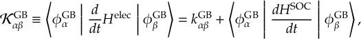
|
(8.51) |
where GB denotes that this is a general basis which can be either diagonal or MCH representation, superscript SOC denotes the spin-orbit coupling terms, and
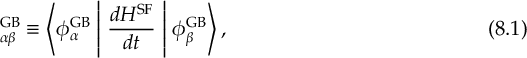
|
(8.52) |
where superscript SF denotes spin-free.
One can show that,
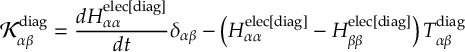
|
(8.53) |
and

|
(8.54) |
Similar as in the NGT scheme, we now neglect [d/dt]HSOC. This gives the TDM scheme
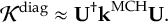 |
(8.55) |
Therefore,
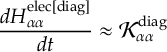
|
(8.56) |
and

|
(8.57) |
This is very useful, because it allows us to compute [(dHelec[diag]αα)/dt] without computing nonadiabatic coupling vectors.
One can show that the only requirement a diagonal gradient needs to be fulfilled to conserve energy is,
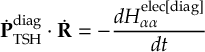
|
(8.58) |
where · PdiagTSH is the diagonal force. Therefore, by knowing [(dHelec[diag]αα)/dt] one can obtain an alternative energy conserving force as
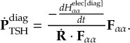
|
(8.59) |
The above diagonal force conserves energy for any real and nonzero vector Fαα that is not normal to · R. In SHARC3.0, we use the following physically motivated choice of Fαα
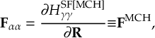
|
(8.60) |
where state γ is a state in the MCH basis that corresponds to state α in the diagonal basis.
In SHARC3.0, the default is to use different approaches to compute [(dHelec[diag]αα)/dt] for different algorithms. For overlap-based algorithms,
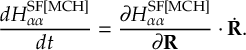
|
(8.61) |
This defines kMCH for overlap-based algorithm, and one transform kMCH to Kdiag with equation (8.55). This is called gradient approach, and can be turned on by using keyword tdm_method gradient.
The default for curvature-driven algorithms is that we employ finite differences to compute both [(dHSF[MCH]αα)/dt] and [(dHelec[diag]αα)/dt]. For the first and second time steps, we use first-order backward finite differences
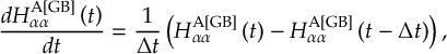
|
(8.62) |
where superscript A can be SOC, SF, or elec (full Hamiltonian, includong both SF and SOC).
And for later steps, we use second-order backward finite differences

|
(8.63) |
This is called the energy approach, and can be turned on by using keyword tdm_method energy.
8.11.3 Dipole moment derivatives
For strong laser fields, the derivative of the dipole moments might be a non-negligible contribution to the gradients. In this case, they should be included in the gradient transformation step:
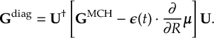
|
(8.64) |
This can be activated with the keyword dipole_grad in the SHARC input file.
8.12 Internal coordinates definitions
In this section, the internal coordinates available in geo.py are defined.
Bond length
The bond length between two atoms a and b is:
|
(8.65) |
Bond angle
The bond angle for atoms a, b and c is defined as the angle
 |
(8.66) |
where vba is the vector from atom b to atom a.
Dihedral
The dihedral angle is defined via the vectors w1 and w2:

|
(8.67) |
The dihedral is given as the angle between w1 and w2 according to equation (8.66).
In order to distinguish left- and right-handed rotation, also the vector Q=w1×w2 is computed, and if the angle between Q and vbc is larger than 90° then the value of the dihedral is multiplied by -1.
Pyramidalization angle
The pyramidalization angle is defined via the vectors vba and
|
(8.68) |
The pyramidalization angle is then given as 90° − θ(vba,w1).
This definition of the pyramidalization angle works best for nearly planar arrangements, like in amino groups.
An alternative definition of the pyramidalization angle works better for strongly pyramidalized situations (e.g., fac-arranged atoms in a octahedral metal complex).
This pyramidalization angle is defined as 180° minus the angle between vab and the average of vbc and vbd.
Cremer-Pople parameters
The definitions of the Cremer-Pople parameters for 5- and 6-membered rings is described in [66].
Boeyens classification
For 6-membered rings, the Boeyens classification scheme is described in [67].
Angle between two rings
In order to compute angles between the mean planes of two rings, we compute the normal vector of the two rings as in [66].
We then compute the angle between the two normal vectors.
8.13 Kinetic energy adjustments
There are several options how to adjust the kinetic energy after a surface hop occurred. The simplest option is to not adjust the kinetic energy at all (input: ekincorrect none), but this obviously leads to violation of the conservation of total energy.
Alternatively, the velocities of all atoms can be rescaled so that the new kinetic energy and the potential energy of the new state β again sum up to the total energy.
|
(8.69) |

|
(8.70) |
|
(8.71) |
Within this methodology, when the energy of the old state α was lower than the energy of the new state β the kinetic energy is lowered. Since the kinetic energy must be positive, this implies that there might be states which cannot be reached (their potential energy is above the total energy). A hop to such a state is called “frustrated hop” and will be rejected by SHARC. Rescaling parallel to the nuclear velocity vector is requested with ekincorrect parallel_vel.
Alternatively, according to Tully’s original formulation of the surface hopping method [14], after a hop from α to β only the component of the velocity along the direction of the nonadiabatic coupling vector Kβα should be rescaled. With[126]
|
(8.72) |
|
(8.73) |
the available energy can be calculated:
|
(8.74) |
If ∆ < 0, the hop is frustrated and will be rejected. Otherwise, the scaled velocities v′ can be calculated as
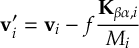
|
(8.75) |
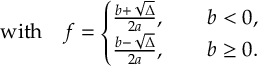
|
(8.76) |
This procedure can be requested with ekincorrect parallel_nac. Note that in this case SHARC will request the nonadiabatic coupling vectors, even if they are not used for the wave function propagation.
8.13.1 Reflection for frustrated hops
As suggested by Tully [14], during a frustrated hop one might want to reflect the trajectory (i.e., invert some component of the velocity vector).
In SHARC, there are three possible options to this, the first being no reflection (reflect_frustrated none).
Alternatively, one can invert the total velocity vector v:=−v (reflect_frustrated parallel_vel).
As this leads to a nearly complete time reversal and might be inappropriate, as a third option one can choose to only reflect the velocity component parallel to the nonadiabatic coupling vector between the active state and the state to which the frustrated hop was attempted.
The condition for reflection in this case is based on three scalar products:
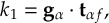
|
(8.77) |
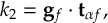
|
(8.78) |
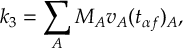
|
(8.79) |
Reflection is only carried out if k1k2 < 0 and k2k3 < 0.
In order to reflect, we compute:
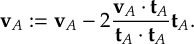
|
(8.80) |
where tA is the component of tαf corresponding to atom A.
8.13.2 Choices of momentum adjustment direction
In addition to previously mentioned choices of vectors to adjustment momentum, namely, velocity vector, and nonadiabatic coupling vector, in SHARC3.0 we have several new choices of momentum adjustment vectors. A complete list includes: velocity vector,
projected velocity vector (vibrational velocity vector),
nonadiabatic coupling vector,
projected nonadiabatic coupling vector,
difference gradient vector,
effective nonadiabatic coupling vector,
and projected effective nonadiabatic coupling vector.
Note that using the projected vectors is recommended choice because these vectors can conserve angular momentum and center of mass motion. Section 8.31 introduces the effective nonadiabatic coupling vector, and Section 8.14 introduces the projection operator.
Section 8.34 distinguishes different types of nonadiabatic dynamics algorithms based on the coupling types to be computed. Although using nonadiabatic coupling vector as momentum adjustment direction is most accurate, one of the advantages of not using nonadiabatic coupling vector as momentum adjustment direction is that one can utilize the advantages of overlap-based algorithms and curvature-driven algorithms that nonadiabatic coupling vector is not needed in propagating electronic and nuclear equations of motion.
8.14 Projection operator
The projection operator projects out the translational and rotational components of a vector, i.e., nonadiabatic coupling vector (NAC vector). The projected NAC, is expressed as
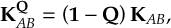
|
(8.81) |
where 1 and Q are the identity operator and projection operator, respectively, and A and B are indices of electronic states.
The projection operator is a 3N×3N matrix with elements

|
(8.82) |
where indices i and i’ label the nuclei and vary from 1 to N, α, β, γ, α‘, β‘, and γ‘ take on the values x, y, and z.
~I −1 is the inverse of matrix ~I.
Matrix ~I is same as moment of inertia matrix with all masses set to 1, and \varepsilonup is the completely antisymmetric third-order unit pseudotensor, whose elements are the Levi-Civita symbols.
The first term of the projection operator projects onto the three directions corresponding to overall translation, and the second term projects onto the three directions corresponding to overall rotation.
8.15 Fewest switches with time uncertainty
The fewest switches with time uncertainty (FSTU) propagation is identical to the FS algorithm except when there is a frustrated hop. The FSTU looks for nonlocal hops to reduce the number of frustrated hops.
At time t, the FSTU algorithm computes the potential energy differences between the active state K and the rest of the states,

|
(8.83) |
where Vα(t) is the adiabatic potential energy of state α at time t. In SHARC3.0, the velocity is rescaled after a K→ α hop according to
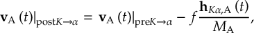
|
(8.84) |
where vA, hKα,A, and MA are respectively the velocity vector, momentum adjustment vector, and the atomic mass of atom A, and f is a unitless factor to be computed.
The factor f is computed by requiring energy conservation after a hop

|
(8.85) |
Therefore,
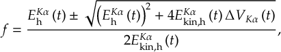
|
(8.86) |
where
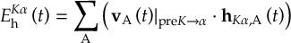
|
(8.87) |
and
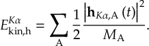
|
(8.88) |
To have a real solution of f, the following condition must be fulfilled:
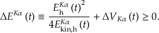
|
(8.89) |
At time t0, when one encounters a K→ β hop that is frustrated by the FS algorithm, one computes the FSTU uncertainty time for this unconfirmed hop as
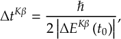
|
(8.90) |
where the absolute value is needed because ∆EKβ(t0) is negative. Then FSTU algorithm looks for energy accessible K→ β hop within this time uncertainty region.
8.16 Laser fields
The program laser.x can calculate laser fields as superpositions of several analytical, possibly chirped, laser pulses. In the following, the laser parametrization is given (see [127] for further details).
8.16.1 Form of the laser field
In general, the laser field ϵ(t) is a linear superposition of a number of laser pulses li(t):
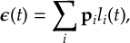
|
(8.91) |
where pi is the normalized polarization vector of pulse i.
A pulse l(t) is formed as the product of an envelope function and a field function.
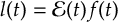
|
(8.92) |
8.16.2 Envelope functions
There are two types of envelope function defined in laser.x, which are Gaussian and sinusoidal.
The Gaussian envelope is defined as:
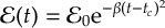 |
(8.93) |
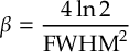 |
(8.94) |
where E0 is the peak field strength, FWHM is the full width at half maximum and tc is the temporal center of the pulse.
The sinusoidal envelope is defined as:
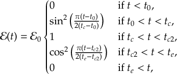 |
(8.95) |
where again E0 is the peak field strength, t0 and tc define the interval where the field strength increases, and tc2 and te define the interval where the field strength decreases. Figure 8.3 shows the general form of the envelope functions and the meaning of the temporal parameters t0, tc, t2c and te.
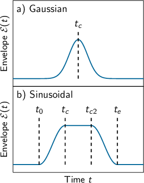
8.16.3 Field functions
The field function f(t) is defined as:
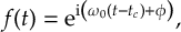
|
(8.96) |
where ω0 is the central frequency and ϕ is the phase of the pulse. Even though the laser field is complex in this expression, in the propagation of the electronic wave function in SHARC only the real part is used.
8.16.4 Chirped pulses
In order to apply a chirp to the laser pulse l(t), it is first Fourier transformed to the frequency domain, giving the function ~l(ω). The chirp is applied by calculating:
 |
(8.97) |
The chirped laser in the time domain l′(t) is then obtained by Fourier transform of the chirped pulse ~l′(ω).
8.16.5 Linear chirp without Fourier transform
If laser.x was compiled without the FFTW package, the only accessible chirps are linear chirps for Gaussian pulses:

|
(8.98) |

|
(8.99) |
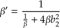
|
(8.100) |
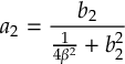
|
(8.101) |
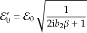
|
(8.102) |
Other chirps are only possible with the Fourier transformation.
8.17 Laser interactions
The laser field ϵ is included in the propagation of the electronic wave function. In each substep of the propagation, the interaction of the laser field with the dipole moments is included in the Hamiltonian. The contribution Vi is in each time step added to the Hamiltonian in equations (8.193) or (8.198), respectively:
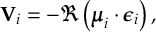
|
(8.103) |
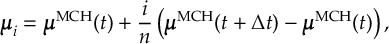
|
(8.104) |
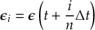
|
(8.105) |
where i, n t and ∆t are defined as in section 8.33.
8.17.1 Surface Hopping with laser fields
If laser fields are present, there can be two fundamentally different types of hops: laser-induced hops and nonadiabatic hops. The latter ones are the same hops as in the laser-free simulations, and demand that the total energy is conserved. The laser-induced hops on the other hand demand that the momentum (kinetic energy) is conserved. Hence, SHARC needs to decide for every hop whether it is laser-induced or not.
Consider a previous state α and a new state β. Currently, the hop is classified based on the energy gap ∆E=|Eβdiag−Eαdiag| and the instantaneous central energy of the laser pulse ω.
The hop is assumed to be laser-induced if
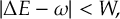
|
(8.106) |
where W is a fixed parameter. W can be set using the input keyword laserwidth.
If a hop has been classified as laser-free, the momentum is adjusted according to the equations given in section 8.13.
8.18 Linear/Quadratic Vibronic Coupling Models
In the vibronic coupling model [116] the diabatic energy and coupling matrix V is constructed as
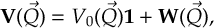 |
(8.107) |
where V0(→Q) is the reference potential and W(→Q) includes the state-specific vibronic terms.
Within SHARC, the reference potential is chosen to be a harmonic oscillator.
The reference potential is expressed in dimensionless mass-frequency-scaled normal coordinates, which can be computed from the Cartesian coordinates rA as
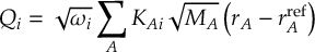 |
(8.108) |
where ωi is the frequency of normal mode i, MA is an atomic mass, and KA i denotes the conversion matrix between mass-weighted Cartesian and normal coordinates.
Using these coordinates, the harmonic reference potential is given as
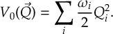 |
(8.109) |
In the case of the quadratic vibronic coupling model, one additionally considers the following state-specific terms that constitute the W matrix.
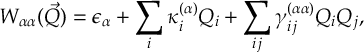 |
(8.110) |
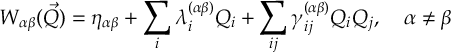 |
(8.111) |
Here the ϵα are the vertical excitation energies, the ηαβ are the SOC constants, and the κi(α) and λi(αβ) are termed intrastate and interstate linear vibronic coupling constant [116].
The γij(αβ) terms are quadratic vibronic coupling constants, where there are different types (inter/intra-state as well as quadratic/bilinear).
Within SHARC4, the SOCs can also have a linear dependence:
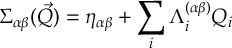
|
(8.112) |
These are called lambda_soc in the LVC.template file.
Also within SHARC4, one can use LVC in the presence of solvent point charges, in an electrostatic embedding fashion [36].
Here, a solvent-charge-dependent term is added to W (including the diagonal αα):
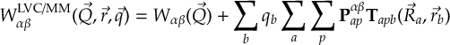
|
(8.113) |
where →r is the vector of the point charge coordinates, →q collects the point charge values, and the sum is evaluated in real space, not in normal mode coordinates (therefore the equation shows →R rather than →Q).
Here, T is the geometric tensor [36] that is computed from the positions of all involved atoms, and Pαβ is the tensor of the multipole charges for the state density (αα) or transition density (αβ).
For each αβ, there are 10natom multipole charges.
Note that the solvent-dependent term is computed considering the relative orientation of the current and reference geometry, by means of the Kabsch algorithm.
8.18.1 Obtaining LVC parameters from ab initio data
All LVC parameters are either constant or linear, implying that they can be obtained from either a single ab initio computation or from some first derivative.
The following equations show how the parameters ϵα, ηαβ, κi(α), and λi(αβ) are obtained.
The parameters ϵα are simply the vertical excitation energies at the reference geometry:

|
(8.114) |
where Eref is some reference energy.
Likewise, the SOC parameters ηαβ are simply the SOC matrix elements at the reference geometry:
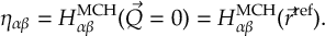
|
(8.115) |
These two equations hold because in the LVC model we assume that at the reference geometry diabatic basis and MCH basis coincide.
The intrastate linear vibronic coupling term κi(α) is the gradient of the diabatic energy of state n.
Since at the reference geometry, diabatic and MCH basis coincide, this is equivalent to the gradient of the corresponding MCH state.
This gradient needs only be transformed from Cartesian coordinates into normal mode coordinates:
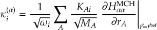
|
(8.116) |
The interstate linear vibronic coupling term λi(αβ) is the gradient of the diabatic coupling between states n and m.
If analytical nonadiabatic coupling vectors are available, these parameters can be obtained-similarly as the κi(α) parameters-by coordinate transformation of the energy-difference-scaled nonadiabatic coupling vector:
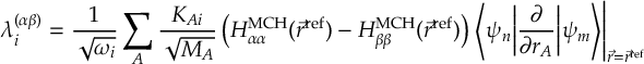
|
(8.117) |
If gradients or nonadiabatic coupling vectors are not available, then the κi(α) and λi(αβ) parameters can be obtained numerically.
To this end, one performs ab initio calculations at displaced geometries ±δQi, where
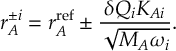
|
(8.118) |
The ab initio calculations at these geometries provide the energies HMCHαα(rA±i) and the wave function overlaps S±iαβ=〈ψMCHα(→rref)|ψMCHβ(→r±i)〉.
From these data, the κi(α) values can be computed as:

|
(8.119) |
and the λi(αβ) as:

|
(8.120) |
The Λ(αβ)i terms are evaluated similarly from the diabatized SOCs.
The multipolar charges are evaluated by means of a RESP fit; the diabatic multipolar charges in the LVC template file are assumed identical to the charges at the reference geometry.
8.19 Normal Mode Analysis
The normal mode analysis can be used to find important vibrational modes in the excited-state dynamics.[68,[69]
Given a matrix Q containing the normal mode vectors and a reference geometry Rref, calculate for each trajectory
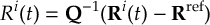
|
(8.121) |
to obtain the displacements in normal mode coordinates.
Averaging over the displacements gives the average trajectory:
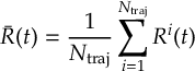
|
(8.122) |
which should contain only coherent motion, since random motion cancels out in an ensemble.
A measure for the coherent activity in a mode is the standard deviation (over time) of the average trajectory:

|
(8.123) |
where kstart and kend are the start and end time steps for the analysis.
Rcoh a vector with one number per normal mode, where larger number mean that there is more coherent activity in this mode.
A measure for the total motion in a mode is the total standard deviation:
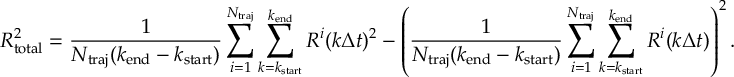
|
(8.124) |
8.20 Optimization of Crossing Points
With orca_External it is possible to optimize different kinds of crossing points.
In all cases, these optimizations involve the energies of the lower state El and upper state Eu, the energy difference ∆E=Eu−El, the gradients of the lower state gl and upper state gu, the gradient difference vector d, and/or the nonadiabatic coupling vector t.
The simplest case is the optimization of minimum-energy crossing points between states of different multiplicity, because in this case the nonadiabatic coupling vector is zero and the branching space is one-dimensional.
In this case [72], the energy to optimize is Eu inside the intersection space, and ∆E inside the branching space.
The corresponding gradient to follow F can be written as:
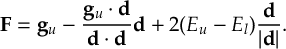
|
(8.125) |
More complicated is the optimization of a conical intersection, between states of the same multiplicity, because the branching space is two-dimensional.
The corresponding gradient to follow F is:
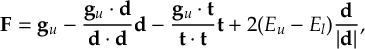
|
(8.126) |
where d and t need to be orthogonalized.
If no nonadiabatic coupling vector is available because the interface cannot deliver them, conical intersections are optimized with the penalty function method of Levine et al. [73].
The effective energy to optimize is defined as:
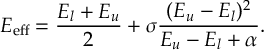
|
(8.127) |
This equation is a combination of the two main targets of the optimization, the average energy and the energy gap.
The parameter σ allows prioritizing either of the two, with a larger σ leading to smaller energy gaps.
The parameter α is there to avoid the discontinuity at Eu=El.
The corresponding gradient to follow F is:
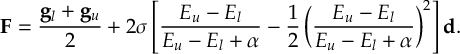
|
(8.128) |
Note that σ and α might strongly influence the quality (i.e., with the penalty function method the optimization will not converge to the true minimum energy conical intersection point) of the result and the convergence behavior.
A large σ and a small α will improve the quality of the result, but make the optimization harder to converge.
8.21 Phase tracking
8.21.1 Phase tracking of the transformation matrix
A Hermitian matrix HMCH can always be diagonalized. Its eigenvectors form the rows of a unitary matrix U, which can be used to transform between the original basis and the basis of the eigenfunctions of H.
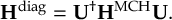
|
(8.129) |
However, the condition that U diagonalizes HMCH is not sufficient to define U uniquely. Each normalized eigenvector u can be multiplied by a complex number on the unit circle and still remains a normalized eigenvector.

|
(8.130) |
leads to

|
(8.131) |
and
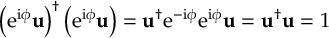
|
(8.132) |
Thus, for all diagonal matrices Φ with elements
δβαexp(iϕβ),
also the matrix U′=UΦ diagonalizes HMCH (if U diagonalizes it).
The propagation of the coefficients in the diagonal basis is written as (see section 8.33):
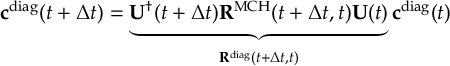
|
(8.133) |
where U(t) and U(t+∆t) are determined independently from diagonalizing the matrices HMCH(t) and HMCH(t+∆t), respectively. However, depending on the implementation of the diagonalization, U(t) and U(t+∆t) may carry unrelated, random phases. Even if HMCH(t) and HMCH(t+∆t) were identical, U(t) and U(t+∆t) might still differ, e.g.:
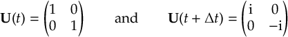
|
(8.134) |
The result is that the coefficients c pick up random phases during the propagation, leading to random changes in the direction of population transfer, invalidating the whole propagation.
In order to make the phases of U(t) and U(t+∆t) as similar as possible, SHARC employs a projection technique. First, we define the overlap matrix V between U(t) and U(t+∆t):
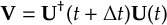
|
(8.135) |
For ∆t=0, clearly
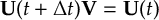
|
(8.136) |
and V can be identified with the phase matrix Φ.
For ∆t ≠ 0, we must now find a matrix P so that
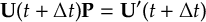
|
(8.137) |
still diagonalizes HMCH(t+∆t), but which minimizes the phase change with regard to U(t).
The matrix P has elements
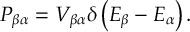
|
(8.138) |
where Eβ is the β-th eigenvalue of HMCH(t+∆t).
Within the SHARC algorithm, the phase of U(t+∆t) is adjusted to be most similar to U(t) by calculating first V, generating P from V and the eigenvalues of HMCH(t+∆t) and calculating the phase-corrected matrix U′(t+∆t) as U(t+∆t)P.
8.21.2 Tracking of the phase of the MCH wave functions
Additionally, within the quantum chemistry programs, the phases of the electronic wave functions may change from one time step to the next one. This will result in changes of the phase of all off-diagonal matrix elements (spin-orbit couplings, transition dipole moments, nonadiabatic couplings). SHARC has several possibilities to correct for that:
- The interface can provide wave function phases through QM.out.
- If the overlap matrix is available, its diagonal contains the necessary phase information.
- Otherwise the scalar products of old and new nonadiabatic couplings and the relative phase of SOC matrix elements can be used to construct phase information.
8.22 Random initial velocities
Random initial velocities are calculated with a given amount of kinetic energy E per atom a. For each atom, the velocity is calculated as follows, with two uniform random numbers θ and ϕ, from the interval [0,1[:
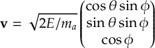
|
(8.139) |
This procedure gives a uniform probability distribution on a sphere with radius √{2E/ma}.
Note that the translational and rotational components of random initial velocities are not projected out in the current implementation.
Random initial velocities can be requested in the input with veloc random E, where E is a float defining the kinetic energy per atom (in eV).
8.23 Representations
Within SHARC, two different representations for the electronic states are used. The first is the so-called MCH basis, which is the basis of the eigenfunctions of the molecular Coulomb Hamiltonian. The molecular Coulomb Hamiltonian is the standard electronic Hamiltonian employed by the majority of quantum chemistry programs. It contains only the kinetic energy of the electrons and the potential energy arising from the Coulomb interaction between the electrons and nuclei.

|
(8.140) |
With this hamiltonian, states of the same multiplicity couple via the nonadiabatic couplings, while states of different multiplicity do not interact at all.
The second representation used in SHARC is the so-called diagonal representation. It is the basis of the eigenfunctions of the total Hamiltonian.
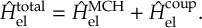
|
(8.141) |
The term ∧Helcoup contains additional couplings not contained in the molecular Coulomb Hamiltonian. The most common couplings are spin-orbit couplings and interactions with an external electric field.
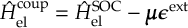
|
(8.142) |
Both of these couplings introduce off-diagonal elements in the total Hamiltonian. Thus, the eigenfunctions of the molecular Coulomb Hamiltonian are not the eigenfunctions of the total Hamiltonian.
Within SHARC, usually quantum chemistry information is read in the MCH representation, while the surface hopping is performed in the diagonal one.
8.23.1 Current state in MCH representation
Oftentimes, it is very useful to know to which MCH state the currently active diagonal state corresponds. If ∧Helcoup is small or the state separation is large, then each diagonal state approximately corresponds to one MCH state. Only in the case of large couplings and/or near-degenerate states are the MCH states strongly mixed in the diagonal states.
In order to obtain for a given time step from the currently active diagonal state β the corresponding MCH state α, a vector cdiag with cidiag=δiβ is generated. The vector is transformed into the MCH representation
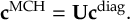
|
(8.143) |
The corresponding MCH state α is the index of the (absolute) largest element of vector cMCH.
8.24 Sampling from Wigner Distribution
The sampling is based on references [59,[60].
Besides the equilibrium geometry Req, the optimization plus frequency calculation provides a set of vibrational frequencies {νi} and the corresponding normal mode vectors {ni}, where i runs from 1 to N=3natom.
The normal mode vectors need to be provided in terms of mass-weighted Cartesian normal modes, in atomics units (Bohrs times square root of electron mass, i.e., a0·√{me}).
Most quantum chemistry programs follow different conventions when writing MOLDEN files. MOLPRO and MOLCAS write these files with unweighted Cartesian normal modes, with units of a0 (Bohrs). GAUSSIAN, TURBOMOLE, Q-CHEM, ADF, and ORCA employ what could be called the ” GAUSSIAN convention”, which are normalized Cartesian normal modes. COLUMBUS uses yet another convention in the output of their suscal.x module.
The script wigner.py automatically transforms these different conventions; it does so by applying all possible transformations to the input data until it finds one transformation which produces an orthonormal normal mode matrix.
The latter one is then used for the Wigner sampling.
In order to create an initial condition (R,v), the following procedure is applied. Initially, R0=Req and v0=0. Then, for each normal mode i, two random numbers Pi and Qi are chosen uniformly from the interval [−5,5]. The value of a ground state quantum Wigner distribution for these values is calculated:
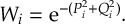
|
(8.144) |
Wi is compared to a uniform random ri number from [0,1]. If Wi > ri, then Pi and Qi are accepted.
Subsequently, the coordinates:
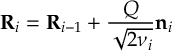 |
(8.145) |
and velocities
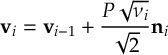 |
(8.146) |
are updated.
The random number procedure and updates are repeated for all normal modes, until (RN,v)N is obtained, which constitutes one initial condition. Finally, the center of mass is restored and translational and rotational components are projected out of v. The harmonic potential energy is given by:
|
(8.147) |
8.24.1 Sampling at Non-zero Temperature
In the case of a non-zero temperature, the molecule might not be in the vibrational ground state of the harmonic oscillator, but rather in an excited vibrational state.
For a given mode i, the probability to be in any given vibrational state j (j=0 is the ground state) is:
|
(8.148) |
where y is νi divided by kBT.
In order to find the vibrational state for mode i, a random number is drawn (from [0,1]) and used as in equation (8.154).
The displacements and velocity contributions for mode i in state j are then obtained as in equations (8.145) and (8.146), except that the Wigner distribution for state j is calculated as:
|
(8.149) |
8.25 Scaling
The scaling factor (keyword scaling) applies to all energies and derivatives of energies. Hence, the full Hamiltonian is scaled, and the gradients are scaled. Nothing else is scaled (no dipole moments, nonadiabatic couplings, overlaps, etc).
8.26 Seeding of the RNG
The standard Fortran 90 random number generator (used for sharc.x, but not for the auxiliary scripts) is seeded by a sequence of integers of length n, where n depends on the computer architecture. The input of SHARC, however, takes only a single RNG seed, which must reproducibly produce the same sequence of random numbers for the same input.
In order to generate the seed sequence from the single input x, the following procedure is applied:
- Query for the number n,
- Generate a first seed sequence s with si=x+37i+17i2,
- Seed with the sequence s,
- Obtain a sequence r of n random numbers on the interval [0,1[,
- Generate a second seed sequence s′ with si′=int(65536(ri−[1/2])),
- Reseed with the sequence s′.
The fifth step will generate a sequence of nearly uncorrelated numbers, distributed uniformly over the full range of possible integer values.
8.27 Selection of gradients and nonadiabatic couplings
In order to increase performance, it is possible to omit the calculation of certain gradients and nonadiabatic couplings. An energy-gap-based algorithm selects at each time step a subset of all possible gradients and nonadiabatic couplings to be calculated. Given the diagonal energy Ediagξ of the current active state ξ, the gradient gMCHα of MCH state α is calculated if:
|
(8.150) |
where εgrad is the selection threshold.
Similarly, a nonadiabatic coupling vector KMCHβα is calculated if:

|
(8.151) |
with selection threshold εnac.
Neither gMCHα nor KMCHβα are ever calculated if α or β are frozen states.
There is only one keyword (eselect) to set the selection threshold, so εgrad and εnac are the same in most cases.
8.28 State ordering
The canonical ordering of MCH states of different S and MS in SHARC is as follows. In the innermost loop, the quantum number is increased; then MS and finally S. Example:
nstates 3 0 3
In this example, the order of states is given as:
| Number | Label | S | MS | n |
| 1 | S0 | 0 | 0 | 1 |
| 2 | S1 | 0 | 0 | 2 |
| 3 | S2 | 0 | 0 | 3 |
| 4 | T1− | 2 | -1 | 1 |
| 5 | T2− | 2 | -1 | 2 |
| 6 | T3− | 2 | -1 | 3 |
| 7 | T10 | 2 | 0 | 1 |
| 8 | T20 | 2 | 0 | 2 |
| 9 | T30 | 2 | 0 | 3 |
| 10 | T1+ | 2 | +1 | 1 |
| 11 | T2+ | 2 | +1 | 2 |
| 12 | T3+ | 2 | +1 | 3 |
The canonical ordering of states is for example important in order to specify the initial state in the MCH basis (using the state keyword in the input file).
Note that the diagonal states do not follow the same prescription. Since the diagonal states are in general not eigenfunctions of the total spin operator, they do not have a well-defined multiplicity.
Hence, the diagonal states are simply ordered by increasing energy.
8.29 Surface Hopping
Given two coefficient vectors cdiag(t) and cdiag(t+∆t) and the corresponding propagator matrix Rdiag(t+∆t,t), the surface hopping probabilities are given by
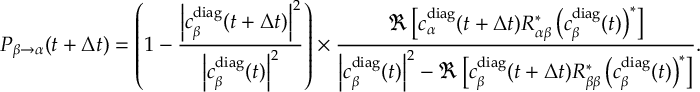
|
(8.152) |
where, however, Pβ→β=0 and all negative Pβ→α are set to zero.
This equation is the default in SHARC, and can be used with hopping_procedure sharc.
Alternatively, the hopping probabilities can be obtained with the “global flux surface hopping” method by Prezhdo and coworkers [55].
The equation is:
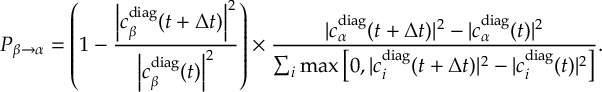
|
(8.153) |
As above, Pβ→β=0 and all negative Pβ→α are set to zero.
This equation and can be used with hopping_procedure gfsh.
In any case, the hopping procedure itself obtains a uniform random number r from the interval [0,1]. A hop to state α is performed, if
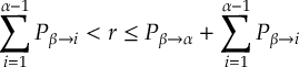 |
(8.154) |
See section 8.13.1 for further details on how frustrated hops (hops according to the hopping probabilities, but where not enough energy is available to execute the hop) are handled.
8.30 Self-Consistent Potential Methods
In trajectory surface hopping (TSH) methods, the trajectory is propagating on a single potential energy surface at each segment of time. Contrary, in the self-consistent potential (SCP) methods, trajectories are propagating on a SCP which is an äveraged” potential. The SCP methods are also self-consistent in terms of electronic and nuclear equations of motion (EOMs), and therefore, does not suffer from the notorious frustrated hops problem of TSH. The starting point of advanced SCP methods like CSDM is semiclassical Ehrenfest (SE), which is derivable from the time-dependent Schrödinger equation (TDSE).
Consider a wave function that is a product of electronic and nuclear wave functions

|
(8.155) |
Inserting the above molecular wave function into the TDSE, employing the independent trajectory approximation, and treating electrons as quantum particles by expanding the electronic wave function in a general basis (GB),
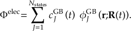
|
(8.156) |
With some mathematical manipulation, one obtains the equation of motion of generalized semiclassical Ehrenfest (GSE) dynamics. The electronic equation of motion of GSE is identical to that of surface hopping,
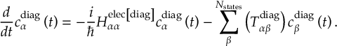
|
(8.157) |
Nuclear equation of motion involves two terms, namely, the adiabatic force and nonadiabatic force.
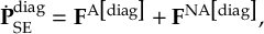
|
(8.158) |
where adiabatic force and nonadiabatic force are, respectively,
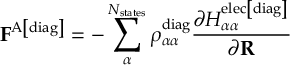
|
(8.159) |
and
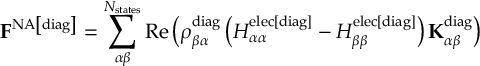
|
(8.160) |
where Kαβdiag is the nonadiabatic coupling vector (NAC). Alternatively, one can use an effective nonadiabatic coupling vector (effective NAC), Gαβ, which is defined as a combination of the difference gradient vector and the velocity vector:
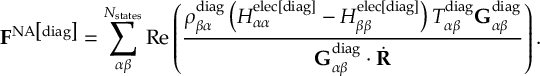
|
(8.161) |
8.30.1 Decoherence in SCP methods
Whereas TSH dynamics involve the coherent propagation of a trajectory on a single potential energy surface, which is stochastically switched, SCP methods include decoherence by considering a combination of coherent and decoherent propagation of a trajectory on the self-consistent potential. This approach leads to the so-called decay of mixing methods.
In this framework, the electronic equation of motion is:
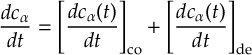
|
(8.162) |
where the coherent term is the same as in the GSE electronic equation of motion (as well as in the TSH equation). The decoherent contribution is introduced to drive the density matrix elements of the state β, which survives to decoherence (called the pointer state), to unity, while all other density matrix elements decay to zero within a relaxation time known as the decoherence time:
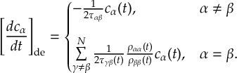 |
(8.163) |
This decoherent term also determines a force in the equation of motion of the nuclei and drives the trajectory to a pure electronic state (i.e., the pointer state):
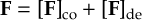
|
(8.164) |
where [ F ]co is identical to the GSE nuclear equation of motion, and the decoherent force contribution is:
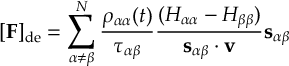
|
(8.165) |
where s is the decoherence vector.[110,[40]
Switchung Procedure
The pointer state is switched during the dynamics with a switching probability that can be computed in three different ways. In the natural decay of mixing (ndm) method [110], the decay of mixing electronic density is used to calculate the switching probability according to the fewest-switches criterion:
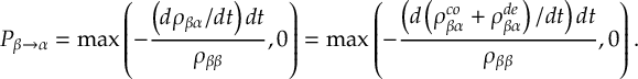
|
(8.166) |
The self-consistent decay of mixing (scdm)[40] method, instead, locally eliminates the decoherent contribution in the electronic density within the switching algorithm:
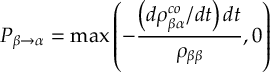
|
(8.167) |
In contrast to scdm, in the coherent switching with decay of mixing (csdm)[30] method, the decoherent contribution to the electronic density matrix used in the switching probability is switched off over an entire region of strong coupling:
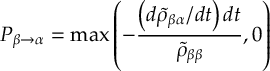
|
(8.168) |
where ~ρβα are the density matrix elements associated to the coherent amplitudes and they are initialized to the decay of mixing quantities (ρβαco + ρβαde) at each local minimum of the coupling strenght defined by:
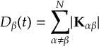
|
(8.169) |
Decoherence Time
The decoherence time in equation (8.163) can be computed using three different approaches. The energy-based decoherence (EDC) correction computes ταβ as:
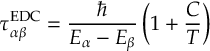
|
(8.170) |
“where T is the total kinetic energy, and C is a parameter usually set to 0.1 Hartree [108]. Alternatively, ταβ can be evaluated in the SCDM framework using the internal vibrational kinetic energy (Tvib) instead of the total kinetic energy:
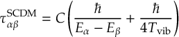
|
(8.171) |
where C is a user-defined parameter, usually set in the range of 6–9 [40].
The csdm method, instead, accounts for momentum constraints in the decoherence process:
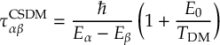
|
(8.172) |
where E0 is 1 Hartree and
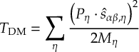
|
(8.173) |
with Pη, ∧sαβ,η, and Mη representing the ηth component of the nuclear momentum, the ηth component of the decoherence direction, and the atomic mass corresponding to the ηth component of the nuclear degree of freedom, respectively.[30]
8.31 Effective Nonadiabatic Coupling Vector
The effective nonadiabatic coupling vector Gαβ is a mixture of difference gradient vector and velocity vector.
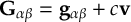
|
(8.174) |
where
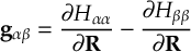
|
(8.175) |
and c is a coefficient. The coefficient c is determined by requiring that the dot product between effective nonadiabatic coupling vector and velocity vector equals time derivative coupling:
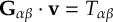
|
(8.176) |
8.32 Velocity Verlet
The nuclear coordinates of atom A are updated according to the Velocity Verlet algorithm [128], based on the gradient of state β at R(t) and R(t+∆t):
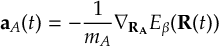
|
(8.177) |
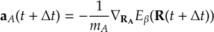
|
(8.178) |
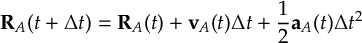
|
(8.179) |
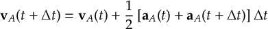
|
(8.180) |
Currently, there are no other integrators for the nuclear motion implemented in SHARC.
8.33 Wavefunction propagation
The electronic wave function is needed in order to carry out surface hopping. The electronic wave function is expanded in the basis of the so-called model space S, which includes the few lowest states |ψMCHα〉 of the multiplicities under consideration (e.g. the 3 lowest singlet and 2 lowest triplet states).
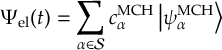
|
(8.181) |
All multiplet components are included explicitly, i.e., the inclusion of an MCH triplet state adds three explicit states to the model space (the three components of the triplet).
Within SHARC, the wave function is represented just by the vector cMCH. The Hamiltonian HMCH is represented in matrix form with elements:
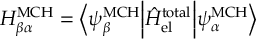
|
(8.182) |
From the MCH representation, the diagonal representation can be obtained by unitary transformation within the model space S (U†HMCHU=Hdiag and U†cMCH=cdiag):
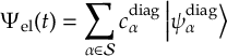
|
(8.183) |
and
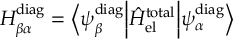
|
(8.184) |
The propagation of the electronic wave function from time t to t+∆t can then be written as the product of a propagation matrix with the coefficients at time t:

|
(8.185) |
or

|
(8.186) |
In order to calculate RMCH(t+∆t,t), SHARC uses (unitary) operator exponentials.
8.33.1 Propagation using nonadiabatic couplings
Here we assume that in the dynamics the interaction between the electronic states is described by a matrix of time-derivative couplings TMCH(t), such that
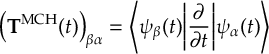 |
(8.187) |
or
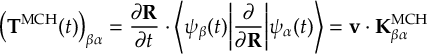 |
(8.188) |
In equation (8.187), the time-derivative couplings are directly calculated by the quantum chemistry program (use coupling ddt in the SHARC input), while in (8.188) the matrix TMCH(t) is obtained from the scalar product of the nuclear velocity and the nonadiabatic coupling vectors (use coupling ddr in the input).
The propagation matrix can then be written as
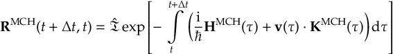
|
(8.189) |
with the time-ordering operator ∧T. For small time steps ∆t, HMCH(τ) and KMCH(τ) can be interpolated linearly

|
(8.190) |
And in order to have a sufficiently small time step for this to work, the interval (t,t+∆t) is further split into subtime steps ∆τ = [(∆t)/n].
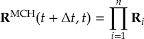
|
(8.191) |
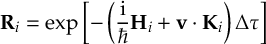
|
(8.192) |
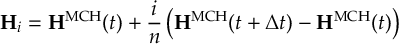 |
(8.193) |

|
(8.194) |
8.33.2 Propagation using overlap matrices – Local diabatization
In many situations, the nonadiabatic couplings in KMCH are very localized on the potential hypersurfaces. If this is the case, in the dynamics very short time steps are necessary to properly sample the nonadiabatic couplings. If too large time steps are used, part of the coupling may be missed, leading to wrong population transfer. The local diabatization algorithm gives more numerical stability in these situations. It can be requested with the line coupling overlap in the input file.
Within this algorithm, the change of the electronic states between time steps is described by the overlap matrix SMCH(t,t+∆t)
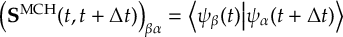 |
(8.195) |
With this, the propagator matrix can be written as
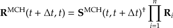
|
(8.196) |
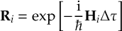
|
(8.197) |
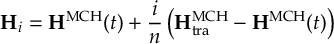 |
(8.198) |

|
(8.199) |
8.33.3 Propagation using overlap matrices – Norm-preserving interpolation
Alternatively, one can use accurate interpolation of time derivative coupling from overlap matrices. Propagating the coefficients can be written as,
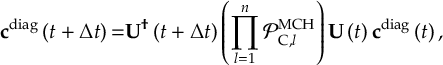
|
(8.200) |
where n is the number of substeps (which can be set up by keyword nsubsteps), and l is the index of substep, with substep propagator PMCHC,l defined as,
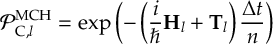
|
(8.201) |
where,

|
(8.202) |
i.e., one linearly interpolates the MCH Hamiltonian Helec[MCH] between time t and t+∆t.
In SHARC3.0, the Tl has variants definitions, and these variants define most of the options available in SHARC3.0 keyword eeom. One can have the following possible definitions:
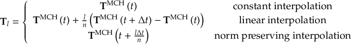
|
(8.203) |
where TMCH(t+[(l∆t)/n]) is the TDC at time t+[(l∆t)/n] which is not computed from electronic structure software, but instead it is from a norm preserving interpolation [107]. During time t and t+∆t, TDC at time T writes
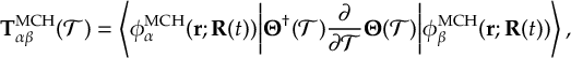
|
(8.204) |
where Θ(T) is a time-dependent transformation matrix that interpolates the MCH (adiabatic) electronic wave functions between time t and t+∆t:
 |
(8.205) |
with
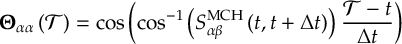
|
(8.206) |
and
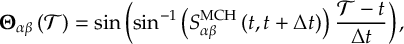
|
(8.207) |
where SMCHαβ is the overlap integral defined in equation equation (8.195).
8.34 Time Derivative Couplings and Curvature Approximation
One of the key ingredients in propagating electronic and nuclear EOMs for GSE and electronic EOM for TSH is time derivative coupling (TDC) in MCH representation. And TDC serves the role as the electronic interstate coupling in the nonadiabatic dynamics. Because TDC cannot be computed directly from electronic structure software, TDC is evaluated by postprocessing quantum chemistry data. There are three ways to compute TDC: NAC-based, overlap-based, and curvature-driven. These three ways of computing TDC corresponds to the three types of algorithms respectively. And controlling the method of TDC evaluation in SHARC3.0 is done by using keyword coupling.
NAC-based TDC
The NAC-based TDC is computed according to equation (8.188), which means a requirement of computing NACs KMCH in MCH representation from quantum chemistry software. Notice that KMCH computational cost scales quadratically as the number of electronic states involved. Therefore it is expensive. In addition, it limits the choices of electronic structure theory, because there is only very limited number of electronic structure theories for which the analytical implementation of NAC is available. Using NAC-based algorithm is enabled by using keyword coupling nacdr or coupling ddr.
Overlap-based TDC
There are three ways to compute overlap-based TDC, all based on overlap integrals defined in equation (8.195).
Therefore, to compute overlap-based TDC, one needs to compute electronic wave functions but not NACs from quantum chemistry software. Tully and Hammes-Schiffer first recognized that TDC can be evaluated based on overlaps. And this is called the Hammes-Schiffer-Tully (HST) scheme of evaluation of TDC from overlaps:

|
(8.208) |
where t is time, and ∆t is the time step. The HST scheme is improved by considering high-order finite difference:

|
(8.209) |
And TDC is most accurately evaluated by a norm-preserving interpolation (NPI) scheme

|
(8.210) |
where TMCHαβ(T) is defined in equation (8.205).
The current implementation of SHARC3.0 employs the NPI scheme to compute overlap-based TDC. However, how TDC is actually used in propagation of electronic EOM is controlled by the keyword eeom and is discussed in section 8.33.
One of the advantages of using NPI scheme over HST or high-order finite difference scheme is that it is more accurate for a situation where the nonadiabatic coupling vector is narrowly peaked (note that NAC is related to TDC), which is often called trivial crossings. It is also more accurate in propagating electronic EOM compared to NAC-based algorithms.
Also notice that the subtle difference between an NPI scheme to evaluate TDCs and the NPI algorithm to propagate electronic EOM. These two are closely related but different.
Using an overlap-based algorithm is enabled by using keyword coupling overlap.
Curvature-driven TDC
The curvature-driven TDC is an approximated TDC that is evaluated from the curvature of potential energy surfaces. Therefore, to compute curvature-driven TDC, one only needs to compute potential energies, neither electronic wave functions nor NACs/overlaps are need from quantum chemistry software. As pointed out by Baeck and An, NAC in a one-dimensional system can be approximated by
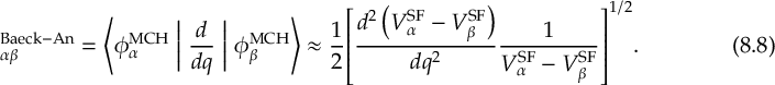
|
(8.211) |
For simplicity we have defined
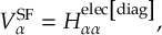
|
(8.212) |
where q is a one-dimensional nuclear coordinate, and we have also adapted the original Baeck and An NAC to the current notation, i.e., the original Baeck and An NAC was considering only for internal conversion processes.
We recognized that a trajectory is in fact propagating on a one-dimensional coordinate which is time. Combining this observation with Baeck and An one-dimensional approximation of NAC gives the definition of curvature-driven TDC (\kappaupTDC)
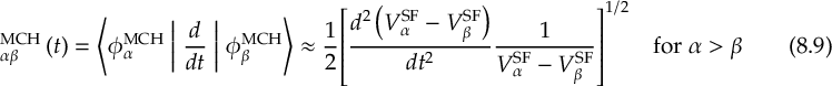 |
(8.213) |
with

|
(8.214) |
Evaluation of the curvature of potential energy with respective to time can be done in two ways, namely by computing first-order differentiation of the time derivative of potential energies from backward finite difference (which is called gradient method), or second-order time derivative of potential energies from backward finite difference (which is called energy method).
We first discuss the gradient method. The gradient method is controlled by using keyword ktdc_method gradient. In the gradient method, we employ the chain rule
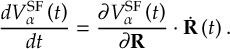
|
(8.215) |
Therefore, (8.213) can be written as
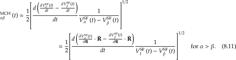 |
(8.216) |
If we define
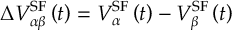
|
(8.217) |
and
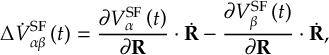 |
(8.218) |
then Equation (8.216) is approximated by backward finite difference as
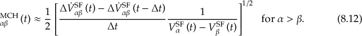 |
(8.219) |
Equations (8.218) and (8.219) define the gradient method. We can see that gradient method requires computation of gradients of all electronic states.
Next we discuss the energy method. The energy method is controlled by using keyword ktdc_method energy. In the energy method, we compute the curvature of potential energy with respective to time directly by backward finite difference as

|
(8.220) |
Starting from the fourth step, we can use

|
(8.221) |
Which method is more practical depends on the details of the simulation.
For TSH without SOCs, only one gradient is needed per time step.
Hence, the gradient method-which requires all gradients-adds significant extra cost and thus for TSH without SOCs it is more convenient to use the energy method.
For TSH with SOCs (and without gradient selection) or for SCP, all gradients are computed anyways, so using the gradient method does not add extra cost.
Thus, the more accurate gradient method is recommended in these cases.
Using the curvature-driven algorithm is enabled by using keyword coupling ktdc. And one can optionally use keyword ktdc_method to select either gradient or energy method to compute \kappaupTDC. Otherwise, the default options for TSH is ktdc_method energy, and for SCP is ktdc_method gradient.
Chapter 9 Bibliography
Bibliography
- [1]
-
M. Kasha:
“”Characterization of
electronic transitions in complex molecules. Discuss. Faraday Soc.,
9, 14 (1950). - [2]
-
C. M. Marian: “”Spin-orbit
coupling and intersystem crossing in molecules. WIREs Comput. Mol.
Sci., 2, 187-203 (2012). - [3]
-
I. Wilkinson, A. E. Boguslavskiy, J. Mikosch, D. M. Villeneuve, H.-J. Wörner,
M. Spanner, S. Patchkovskii, A. Stolow:
“”Non-adiabatic and
intersystem crossing dynamics in SO2 I: Bound State Relaxation Studied
By Time-Resolved Photoelectron Photoion Coincidence Spectroscopy. J.
Chem. Phys., 140, 204 301 (2014). - [4]
-
S. Mai, P. Marquetand, L. González:
“”Non-Adiabatic Dynamics in
SO2: II. The Role of Triplet States Studied by Surface-Hopping
Simulations. J. Chem. Phys., 140, 204 302 (2014). - [5]
-
C. Lévêque, R. Taïeb, H. Köppel:
“”Communication:
Theoretical prediction of the importance of the 3B2 state in the
dynamics of sulfur dioxide. J. Chem. Phys., 140, 091101
(2014). - [6]
-
T. J. Penfold, R. Spesyvtsev, O. M. Kirkby, R. S. Minns, D. S. N. Parker, H. H.
Fielding, G. A. Worth:
“”Quantum dynamics study of
the competing ultrafast intersystem crossing and internal conversion in the
“channel 3” region of benzene. J. Chem. Phys., 137,
204310 (2012). - [7]
-
R. A. Vogt, C. Reichardt, C. E. Crespo-Hernández:
“”Excited-State Dynamics in
Nitro-Naphthalene Derivatives: Intersystem Crossing to the Triplet Manifold
in Hundreds of Femtoseconds. J. Phys. Chem., 117,
6580-6588 (2013). - [8]
-
C. E. Crespo-Hernández, B. Cohen, P. M. Hare, B. Kohler:
“”Ultrafast Excited-State
Dynamics in Nucleic Acids. Chem. Rev., 104, 1977-2020
(2004). - [9]
-
M. Richter, P. Marquetand, J. González-Vázquez, I. Sola, L. González:
“”Femtosecond Intersystem
Crossing in the DNA Nucleobase Cytosine. J. Phys. Chem. Lett.,
3, 3090-3095 (2012). - [10]
-
L. Martínez-Fernández, L. González, I. Corral:
“”An Ab Initio Mechanism
for Efficient Population of Triplet States in Cytotoxic Sulfur Substituted
DNA Bases: The Case of 6-Thioguanine. Chem. Commun., 48,
2134-2136 (2012). - [11]
-
S. Mai, P. Marquetand, M. Richter, J. González-Vázquez, L. González:
“”Singlet and Triplet
Excited-State Dynamics Study of the Keto and Enol Tautomers of Cytosine.
ChemPhysChem, 14, 2920-2931 (2013). - [12]
-
C. Reichardt, C. E. Crespo-Hernández:
“”Ultrafast Spin Crossover
in 4-Thiothymidine in an Ionic Liquid. Chem. Commun., 46,
5963-5965 (2010). - [13]
-
J. C. Tully, R. K. Preston:
“”Trajectory Surface
Hopping Approach to Nonadiabatic Molecular Collisions: The Reaction of
H+ with D2. J. Chem. Phys., 55, 562-572 (1971). - [14]
-
J. C. Tully: “”Molecular
dynamics with electronic transitions. J. Chem. Phys., 93,
1061-1071 (1990). - [15]
-
M. Barbatti: “”Nonadiabatic
dynamics with trajectory surface hopping method. WIREs Comput. Mol.
Sci., 1, 620-633 (2011). - [16]
-
J. E. Subotnik, A. Jain, B. Landry, A. Petit, W. Ouyang, N. Bellonzi:
“”Understanding
the Surface Hopping View of Electronic Transitions and Decoherence.
Annu. Rev. Phys. Chem., 67, 387-417 (2016). - [17]
-
L. Wang, A. Akimov, O. V. Prezhdo:
“”Recent Progress
in Surface Hopping: 2011–2015. J. Phys. Chem. Lett., 7,
2100-2112 (2016). - [18]
-
N. L. Doltsinis: “”Molecular Dynamics Beyond the Born-Oppenheimer
Approximation: Mixed Quantum-Classical Approaches. In J. Grotendorst,
S. Blügel, D. Marx (editors), Computational Nanoscience: Do It
Yourself!, volume 31 of NIC Series, 389-409, John von Neuman
Institut for Computing, Jülich (2006). - [19]
-
N. L. Doltsinis, D. Marx:
“”First Principles
Molecular Dynamics Involving Excited States And Nonadiabatic Transitions.
J. Theor. Comput. Chem., 1, 319-349 (2002). - [20]
-
S. Hammes-Schiffer, J. C. Tully:
“”Proton transfer in
solution: Molecular dynamics with quantum transitions. J. Chem.
Phys., 101, 4657-4667 (1994). - [21]
-
G. Granucci, M. Persico:
“”Critical appraisal of the
fewest switches algorithm for surface hopping. J. Chem. Phys.,
126, 134 114 (2007). - [22]
-
M. Thachuk, M. Y. Ivanov, D. M. Wardlaw:
“”A semiclassical approach
to intense-field above-threshold dissociation in the long wavelength limit.
J. Chem. Phys., 105, 4094-4104 (1996). - [23]
-
B. Maiti, G. C. Schatz, G. Lendvay:
“”Importance of Intersystem
Crossing in the S(3P, 1D) + H2 → SH + H Reaction. J.
Phys. Chem. A, 108, 8772-8781 (2004). - [24]
-
G. A. Jones, A. Acocella, F. Zerbetto:
“”On-the-Fly,
Electric-Field-Driven, Coupled Electron-Nuclear Dynamics. J. Phys.
Chem. A, 112, 9650-9656 (2008). - [25]
-
R. Mitri\’c, J. Petersen, V. Bonac\’c-Koutecký:
“”Laser-field-induced
surface-hopping method for the simulation and control of ultrafast
photodynamics. Phys. Rev. A, 79, 053 416 (2009). - [26]
-
G. Granucci, M. Persico, G. Spighi:
“”Surface hopping
trajectory simulations with spin-orbit and dynamical couplings. J.
Chem. Phys., 137, 22A501 (2012). - [27]
-
B. F. E. Curchod, T. J. Penfold, U. Rothlisberger, I. Tavernelli:
“”Local Control
Theory using Trajectory Surface Hopping and Linear-Response Time-Dependent
Density Functional Theory. Chimia, 67, 218-221 (2013). - [28]
-
G. Cui, W. Thiel:
“”Generalized trajectory
surface-hopping method for internal conversion and intersystem crossing.
J. Chem. Phys., 141, 124 101 (2014). - [29]
-
S. Mai, F. Plasser, P. Marquetand, L. González:
“”General
trajectory surface hopping method for ultrafast nonadiabatic dynamics. In
M. Vrakking, F. Lepine (editors), Attosecond Molecular Dynamics,
chapter 10, 348-385, The Royal Society of Chemistry (2018). - [30]
-
C. Zhu, S. Nangia, A. W. Jasper, D. G. Truhlar:
“”Coherent switching with
decay of mixing: An improved treatment of electronic coherence for
non-Born-Oppenheimer trajectories. J. Chem. Phys., 121,
7658-7670 (2004). - [31]
-
Y. Shu, L. Zhang, S. Mai, S. Sun, L. González, D. G. Truhlar:
“”Implementation of
Coherent Switching with Decay of Mixing into the SHARC Program. J.
Chem. Theory Comput., 16, 3464-3475 (2020). - [32]
-
Y. Shu, L. Zhang, X. Chen, S. Sun, Y. Huang, D. G. Truhlar:
“”Nonadiabatic
Dynamics Algorithms with Only Potential Energies and Gradients:
Curvature-Driven Coherent Switching with Decay of Mixing and Curvature-Driven
Trajectory Surface Hopping. J. Chem. Theory Comput., 18,
1320-1328 (2022). - [33]
-
X. Zhao, I. C. D. Merritt, R. Lei, Y. Shu, D. Jacquemin, L. Zhang, X. Xu,
M. Vacher, D. G. Truhlar:
“”Nonadiabatic
Coupling in Trajectory Surface Hopping: Accurate Time
Derivative Couplings by the Curvature-Driven Approximation.
J. Chem. Theory Comput., 19, 6577-6588 (2023). - [34]
-
S. Mausenberger, S. Polonius, S. Mai, L. González:
“”Efficient,
Hierarchical, and Object-Oriented Electronic Structure Interfaces for Direct
Nonadiabatic Dynamics Simulations. Chemarxiv (2025). - [35]
-
F. Plasser, S. Goméz, S. Mai, L. González:
“”Highly efficient surface
hopping dynamics using a linear vibronic coupling model. Phys. Chem.
Chem. Phys., Advance Article, DOI:10.1039/C8CP05 662E (2018). - [36]
-
S. Polonius, O. Zhuravel, B. Bachmair, S. Mai:
“”LVC/MM: A Hybrid
Linear Vibronic Coupling/Molecular Mechanics Model with Distributed
Multipole-Based Electrostatic Embedding for Highly Efficient Surface Hopping
Dynamics in Solution. J. Chem. Theory Comput., 19,
7171–7186 (2023). - [37]
-
S. Polonius, D. Lehrner, L. González, S. Mai:
“”Resolving
Photoinduced Femtosecond Three-Dimensional Solute–Solvent Dynamics through
Surface Hopping Simulations. J. Chem. Theory Comput., 20,
4738–4750 (2024). - [38]
-
J. Pittner, H. Lischka, M. Barbatti:
“”Optimization
of mixed quantum-classical dynamics: Time-derivative coupling terms and
selected couplings. Chem. Phys., 356, 147 – 152 (2009). - [39]
-
A. Jain, E. Alguire, J. E. Subotnik:
“”An Efficient,
Augmented Surface Hopping Algorithm That Includes Decoherence for Use in
Large-Scale Simulations. J. Chem. Theory Comput., 12,
5256-5268 (2016). - [40]
-
C. Zhu, A. W. Jasper, D. G. Truhlar:
“”Non-Born-Oppenheimer
Trajectories with Self-Consistent Decay of Mixing. J. Chem. Phys.,
120 (2004). - [41]
-
M. Ruckenbauer, S. Mai, P. Marquetand, L. González:
“”Revealing Deactivation
Pathways Hidden in Time-Resolved Photoelectron Spectra. Sci. Rep.,
6, 35 522 (2016). - [42]
-
F. Plasser, M. Wormit, A. Dreuw:
“”New tools for the
systematic analysis and visualization of electronic excitations. I.
Formalism. J. Chem. Phys., 141, 024 106 (2014). - [43]
-
F. Plasser, S. A. Bäppler, M. Wormit, A. Dreuw:
“”New tools for the
systematic analysis and visualization of electronic excitations. II.
Applications. J. Chem. Phys., 141, 024 107 (2014). - [44]
-
F. Plasser: “”TheoDORE: A package for theoretical density, orbital
relaxation, and exciton analysis. http://theodore-qc.sourceforge.net (2017). - [45]
-
D. Farkhutdinova, S. Polonius, P. Karrer, S. Mai, L. González:
“”Parametrization of
Linear Vibronic Coupling Models for Degenerate Electronic States. J.
Phys. Chem. A, 129, 2655–2666 (2025). - [46]
-
L. Grünewald, L. van Dam, S. Mai:
“”An Excitation
Strategy for the Initial Condition Generation for Surface Hopping
Trajectories Using Electron-Only Dynamics Including Explicit Laser Pulses.
J. Chem. Theory Comput., 21, 12 741–12 754 (2025). - [47]
-
J. Janos, P. Slavícek, B. F. E. Curchod:
“”Including
Photoexcitation Explicitly in Trajectory-Based Nonadiabatic Dynamics at No
Cost. J. Phys. Chem. Lett., 15, 10 614–10 622 (2024). - [48]
-
F. A. Korsaye, L. González:
“”Gradient-based
Curvature-only Time-derivative Coupling for Surface Hopping and Coherent
Switching with Decay of Mixing: Application to SO2 and Molecular Tully
Models. ChemRxiv, 2026 (2026). - [49]
-
J. Cerezo, F. Santoro:
“”FCclasses3:
Vibrationally‐resolved spectra simulated at the edge of the harmonic
approximation. J. Comput. Chem., 44, 626–643 (2022). - [50]
-
S. Mai, P. Marquetand, L. González:
“”Nonadiabatic dynamics:
The SHARC approach. WIREs Comput. Mol. Sci., 8, e1370
(2018). - [51]
-
S. Mai, B. Bachmair, L. Gagliardi, H.-G. Gallmetzer, L. Grünewald, M. R.
Hennefarth, N. M. Høyer, F. A. Korsaye, S. Mausenberger, M. Oppel,
T. Pitesa, S. Polonius, E. S. Gil, Y. Shu, N. K. Singer, M. X.
Tiefenbacher, D. G. Truhlar, D. Vörös, L. Zhang, L. González:
“”SHARC4.0: Surface Hopping Including Arbitrary Couplings – Program
Package for Non-Adiabatic Dynamics. https://sharc-md.org/ (2025). - [52]
-
M. Richter, P. Marquetand, J. González-Vázquez, I. Sola, L. González:
“”SHARC: Ab Initio
Molecular Dynamics with Surface Hopping in the Adiabatic Representation
Including Arbitrary Couplings. J. Chem. Theory Comput., 7,
1253-1258 (2011). - [53]
-
M. Richter, P. Marquetand, J. González-Vázquez, I. Sola, L. González:
“”Correction to SHARC: Ab
Initio Molecular Dynamics with Surface Hopping in the Adiabatic
Representation Including Arbitrary Couplings. J. Chem. Theory
Comput., 8, 374-374 (2012). - [54]
-
S. Mai, P. Marquetand, L. González:
“”A General Method to
Describe Intersystem Crossing Dynamics in Trajectory Surface Hopping.
Int. J. Quantum Chem., 115, 1215-1231 (2015). - [55]
-
L. Wang, D. Trivedi, O. V. Prezhdo:
“”Global Flux Surface
Hopping Approach for Mixed Quantum-Classical Dynamics. J. Chem.
Theory Comput., 10, 3598-3605 (2014). - [56]
-
G. Granucci, M. Persico, A. Toniolo:
“”Direct Semiclassical
Simulation of Photochemical Processes with Semiempirical Wave Functions.
J. Chem. Phys., 114, 10 608-10 615 (2001). - [57]
-
F. Plasser, G. Granucci, J. Pittner, M. Barbatti, M. Persico, H. Lischka:
“”Surface Hopping Dynamics
using a Locally Diabatic Formalism: Charge Transfer in The Ethylene Dimer
Cation and Excited State Dynamics in the 2-Pyridone Dimer. J. Chem.
Phys., 137, 22A514 (2012). - [58]
-
F. Plasser, M. Ruckenbauer, S. Mai, M. Oppel, P. Marquetand, L. González:
“”Efficient and
Flexible Computation of Many-Electron Wave Function Overlaps. J.
Chem. Theory Comput., 12, 1207 (2016). - [59]
-
J. P. Dahl, M. Springborg:
“”The Morse oscillator
in position space, momentum space, and phase space. J. Chem. Phys.,
88, 4535-4547 (1988). - [60]
-
R. Schinke: Photodissociation Dynamics: Spectroscopy and Fragmentation of
Small Polyatomic Molecules. Cambridge University Press (1995). - [61]
-
M. Barbatti, K. Sen:
“”Effects of different
initial condition samplings on photodynamics and spectrum of pyrrole.
Int. J. Quantum Chem., 116, 762-771 (2016). - [62]
-
M. Barbatti, G. Granucci, M. Persico, M. Ruckenbauer, M. Vazdar,
M. Eckert-Maksi\’c, H. Lischka:
“”The
on-the-fly surface-hopping program system Newton-X: Application to ab
initio simulation of the nonadiabatic photodynamics of benchmark systems.
J. Photochem. Photobiol. A, 190, 228-240 (2007). - [63]
-
J. J. Bajo, J. González-Vázquez, I. Sola, J. Santamaria, M. Richter,
P. Marquetand, L. González:
“”Mixed Quantum-Classical
Dynamics in the Adiabatic Representation to Simulate Molecules Driven by
Strong Laser Pulses. J. Phys. Chem. A, 116, 2800-2807
(2012). - [64]
-
P. Marquetand, M. Richter, J. González-Vázquez, I. Sola, L. González:
“”Nonadiabatic ab initio
molecular dynamics including spin-orbit coupling and laser fields.
Faraday Discuss., 153, 261-273 (2011). - [65]
-
M. Heindl, L. González:
“”Validating
fewest-switches surface hopping in the presence of laser fields. J.
Chem. Phys., 154 (2021). - [66]
-
D. Cremer, J. A. Pople:
“”General definition of
ring puckering coordinates. J. Am. Chem. Soc., 97,
1354-1358 (1975). - [67]
-
J. C. A. Boeyens: “”The
conformation of six-membered rings. J. Cryst. Mol. Struct.,
8, 317 (1978). - [68]
-
L. Kurtz, A. Hofmann, R. de Vivie-Riedle:
“”Ground state normal mode
analysis: Linking excited state dynamics and experimental observables.
J. Chem. Phys., 114, 6151-6159 (2001). - [69]
-
F. Plasser: Dynamics Simulation of Excited State Intramolecular Proton
Transfer. Master’s thesis, University of Vienna (2009). - [70]
-
A. Amadei, A. B. M. Linssen, H. J. C. Berendsen:
“”Essential dynamics
of proteins. Proteins: Struct., Funct., Bioinf., 17,
412-425 (1993). - [71]
-
S. Nangia, A. W. Jasper, T. F. Miller, D. G. Truhlar:
“”Army Ants Algorithm for
Rare Event Sampling of Delocalized Nonadiabatic Transitions by Trajectory
Surface Hopping and the Estimation of Sampling Errors by the Bootstrap
Method. J. Chem. Phys., 120, 3586-3597 (2004). - [72]
-
M. J. Bearpark, M. A. Robb, H. B. Schlegel:
“”A direct
method for the location of the lowest energy point on a potential surface
crossing. Chem. Phys. Lett., 223, 269 (1994). - [73]
-
B. G. Levine, J. D. Coe, T. J. Martínez:
“”Optimizing Conical
Intersections without Derivative Coupling Vectors: Application to Multistate
Multireference Second-Order Perturbation Theory (MS-CASPT2). J.
Phys. Chem. B, 112, 405-413 (2008). - [74]
-
M. Ruckenbauer, S. Mai, P. Marquetand, L. González:
“”Photoelectron spectra of
2-thiouracil, 4-thiouracil, and 2,4-dithiouracil. J. Chem. Phys.,
144, 074 303 (2016). - [75]
-
F. Plasser, L. González:
“”Communication:
Unambiguous comparison of many-electron wavefunctions through their
overlaps. J. Chem. Phys., 145, 021 103 (2016). - [76]
-
S. Gómez, M. Heindl, A. Szabadi, L. González:
“”From Surface
Hopping to Quantum Dynamics and Back. Finding Essential Electronic and
Nuclear Degrees of Freedom and Optimal Surface Hopping Parameters. J.
Phys. Chem. A, 123, 8321–8332 (2019). - [77]
-
B. R. Landry, M. J. Falk, J. E. Subotnik:
“”Communication: The
correct interpretation of surface hopping trajectories: How to calculate
electronic properties. J. Chem. Phys., 139, 211 101
(2013). - [78]
-
J. Westermayr, M. Gastegger, P. Marquetand:
“”Combining
SchNet and SHARC: The SchNarc Machine Learning Approach for Excited-State
Dynamics. J. Phys. Chem. Lett., 11, 3828-3834 (2020). - [79]
-
Y. Shu, L. Zhang, S. Sun, D. G. Truhlar:
“”Time-Derivative
Couplings for Self-Consistent Electronically Nonadiabatic Dynamics.
J. Chem. Theory Comput., 16, 4098-4106 (2020). - [80]
-
Y. Shu, L. Zhang, Z. Varga, K. A. Parker, S. Kanchanakungwankul, S. Sun, D. G.
Truhlar:
“”Conservation of
Angular Momentum in Direct Nonadiabatic Dynamics. J. Phys. Chem.
Lett., 11, 1135-1140 (2020). - [81]
-
Y. Shu, L. Zhang, D. Wu, X. Chen, S. Sun, D. G. Truhlar: “”New Gradient
Correction Scheme for Electronically Nonadiabatic Dynamics Involving Multiple
Spin States. J. Chem. Theory Comput. (2023). - [82]
-
A. W. Jasper, S. N. Stechmann, D. G. Truhlar:
“”Fewest-switches with time
uncertainty: A modified trajectory surface-hopping algorithm with better
accuracy for classically forbidden electronic transitions. J. Chem.
Phys., 116, 5424-5431 (2002). - [83]
-
X. Zhao, Y. Shu, L. Zhang, X. Xu, D. G. Truhlar:
“”Direct
Nonadiabatic Dynamics of Ammonia with Curvature-Driven Coherent Switching
with Decay of Mixing and with Fewest Switches with Time Uncertainty: An
Illustration of Population Leaking in Trajectory Surface Hopping Due to
Frustrated Hops. J. Chem. Theory Comput., 19, 1672-1685
(2023). - [84]
-
A. V. Akimov, O. V. Prezhdo:
“”The PYXAID Program for
Non-Adiabatic Molecular Dynamics in Condensed Matter Systems. J.
Chem. Theory Comput., 9, 4959-4972 (2013). - [85]
-
A. V. Akimov, O. V. Prezhdo:
“”Advanced Capabilities of
the PYXAID Program: Integration Schemes, Decoherence Effects, Multiexcitonic
States, and Field-Matter Interaction. Journal of Chemical Theory and
Computation, 10, 789-804 (2014), pMID: 26580053. - [86]
-
E. J. Baerends, N. F. Aguirre, N. D. Austin, J. Autschbach, F. M. Bickelhaupt,
R. Bulo, C. Cappelli, A. C. T. van Duin, F. Egidi, C. Fonseca Guerra,
A. Förster, M. Franchini, T. P. M. Goumans, T. Heine, M. Hellström,
C. R. Jacob, L. Jensen, M. Krykunov, E. van Lenthe, A. Michalak, M. M.
Mitoraj, J. Neugebauer, V. P. Nicu, P. Philipsen, H. Ramanantoanina,
R. Rüger, G. Schreckenbach, M. Stener, M. Swart, J. M. Thijssen,
T. Trnka, L. Visscher, A. Yakovlev, S. van Gisbergen:
“”The Amsterdam Modeling
Suite. J. Chem. Phys., 162 (2025). - [87]
-
T. Shiozaki: “”BAGEL:
Brilliantly Advanced General Electronic-structure Library. WIREs
Comput. Mol. Sci., 8, e1331 (2018). - [88]
-
H. Lischka, T. Müller, P. G. Szalay, I. Shavitt, R. M. Pitzer, R. Shepard:
“”Columbus – a program
system for advanced multireference theory calculations. WIREs Comput.
Mol. Sci., 1, 191-199 (2011). - [89]
-
M. J. Frisch, G. W. Trucks, H. B. Schlegel, G. E. Scuseria, M. A. Robb, J. R.
Cheeseman, G. Scalmani, V. Barone, G. A. Petersson, H. Nakatsuji, X. Li,
M. Caricato, A. V. Marenich, J. Bloino, B. G. Janesko, R. Gomperts,
B. Mennucci, H. P. Hratchian, J. V. Ortiz, A. F. Izmaylov, J. L. Sonnenberg,
D. Williams-Young, F. Ding, F. Lipparini, F. Egidi, J. Goings, B. Peng,
A. Petrone, T. Henderson, D. Ranasinghe, V. G. Zakrzewski, J. Gao, N. Rega,
G. Zheng, W. Liang, M. Hada, M. Ehara, K. Toyota, R. Fukuda, J. Hasegawa,
M. Ishida, T. Nakajima, Y. Honda, O. Kitao, H. Nakai, T. Vreven,
K. Throssell, J. A. Montgomery, Jr., J. E. Peralta, F. Ogliaro, M. J.
Bearpark, J. J. Heyd, E. N. Brothers, K. N. Kudin, V. N. Staroverov, T. A.
Keith, R. Kobayashi, J. Normand, K. Raghavachari, A. P. Rendell, J. C.
Burant, S. S. Iyengar, J. Tomasi, M. Cossi, J. M. Millam, M. Klene, C. Adamo,
R. Cammi, J. W. Ochterski, R. L. Martin, K. Morokuma, O. Farkas, J. B.
Foresman, D. J. Fox: “”Gaussian16 Revision A.03 (2016), gaussian
Inc. Wallingford CT. - [90]
-
G. Li Manni, I. Fdez. Galván, A. Alavi, F. Aleotti, F. Aquilante,
J. Autschbach, D. Avagliano, A. Baiardi, J. J. Bao, S. Battaglia,
L. Birnoschi, A. Blanco-González, S. I. Bokarev, R. Broer, R. Cacciari,
P. B. Calio, R. K. Carlson, R. Carvalho Couto, L. Cerdán, L. F.
Chibotaru, N. F. Chilton, J. R. Church, I. Conti, S. Coriani,
J. Cuéllar-Zuquin, R. E. Daoud, N. Dattani, P. Decleva, C. de Graaf,
M. G. Delcey, L. De Vico, W. Dobrautz, S. S. Dong, R. Feng, N. Ferré,
M. Filatov(Gulak), L. Gagliardi, M. Garavelli, L. González, Y. Guan,
M. Guo, M. R. Hennefarth, M. R. Hermes, C. E. Hoyer, M. Huix-Rotllant, V. K.
Jaiswal, A. Kaiser, D. S. Kaliakin, M. Khamesian, D. S. King, V. Kochetov,
M. Kro\’snicki, A. A. Kumaar, E. D. Larsson, S. Lehtola, M.-B. Lepetit,
H. Lischka, P. López Ríos, M. Lundberg, D. Ma, S. Mai,
P. Marquetand, I. C. D. Merritt, F. Montorsi, M. Mörchen, A. Nenov,
V. H. A. Nguyen, Y. Nishimoto, M. S. Oakley, M. Olivucci, M. Oppel,
D. Padula, R. Pandharkar, Q. M. Phung, F. Plasser, G. Raggi, E. Rebolini,
M. Reiher, I. Rivalta, D. Roca-Sanjuán, T. Romig, A. A. Safari,
A. Sánchez-Mansilla, A. M. Sand, I. Schapiro, T. R. Scott,
J. Segarra-Martí, F. Segatta, D.-C. Sergentu, P. Sharma, R. Shepard,
Y. Shu, J. K. Staab, T. P. Straatsma, L. K. Sørensen, B. N. C. Tenorio,
D. G. Truhlar, L. Ungur, M. Vacher, V. Veryazov, T. A. Voß, O. Weser,
D. Wu, X. Yang, D. Yarkony, C. Zhou, J. P. Zobel, R. Lindh:
“”The OpenMolcas
Web: A Community-Driven Approach to Advancing Computational Chemistry.
J. Chem. Theory Comput., 19, 6933–6991 (2023). - [91]
-
H.-J. Werner, P. J. Knowles, F. R. Manby, J. A. Black, K. Doll, A. Heßelmann,
D. Kats, A. Köhn, T. Korona, D. A. Kreplin, Q. Ma, T. F. Miller,
A. Mitrushchenkov, K. A. Peterson, I. Polyak, G. Rauhut, M. Sibaev:
“”The Molpro quantum
chemistry package. J. Chem. Phys., 152 (2020). - [92]
-
J. J. P. Stewart: “”MOPAC: A
semiempirical molecular orbital program. Journal of Computer-Aided
Molecular Design, 4, 1–103 (1990). - [93]
-
G. Granucci, M. Persico, D. Accomasso, E. Sangiogo Gil, S. Corni, J. Fregoni,
T. Laino, M. Tesi, A. Toniolo: “”MOPAC-PI: a program for excited
state dynamics simulations based on nonadiabatic trajectories and
semiempirical electronic structure calculations (2024). - [94]
-
E. Aprà, E. J. Bylaska, W. A. de Jong, N. Govind, K. Kowalski, T. P.
Straatsma, M. Valiev, H. J. J. van Dam, Y. Alexeev, J. Anchell, V. Anisimov,
F. W. Aquino, R. Atta-Fynn, J. Autschbach, N. P. Bauman, J. C. Becca, D. E.
Bernholdt, K. Bhaskaran-Nair, S. Bogatko, P. Borowski, J. Boschen, J. Brabec,
A. Bruner, E. Cauët, Y. Chen, G. N. Chuev, C. J. Cramer, J. Daily,
M. J. O. Deegan, T. H. Dunning, M. Dupuis, K. G. Dyall, G. I. Fann, S. A.
Fischer, A. Fonari, H. Früchtl, L. Gagliardi, J. Garza, N. Gawande,
S. Ghosh, K. Glaesemann, A. W. Götz, J. Hammond, V. Helms, E. D. Hermes,
K. Hirao, S. Hirata, M. Jacquelin, L. Jensen, B. G. Johnson, H. Jónsson,
R. A. Kendall, M. Klemm, R. Kobayashi, V. Konkov, S. Krishnamoorthy,
M. Krishnan, Z. Lin, R. D. Lins, R. J. Littlefield, A. J. Logsdail,
K. Lopata, W. Ma, A. V. Marenich, J. Martin del Campo, D. Mejia-Rodriguez,
J. E. Moore, J. M. Mullin, T. Nakajima, D. R. Nascimento, J. A. Nichols,
P. J. Nichols, J. Nieplocha, A. Otero-de-la Roza, B. Palmer, A. Panyala,
T. Pirojsirikul, B. Peng, R. Peverati, J. Pittner, L. Pollack, R. M. Richard,
P. Sadayappan, G. C. Schatz, W. A. Shelton, D. W. Silverstein, D. M. A.
Smith, T. A. Soares, D. Song, M. Swart, H. L. Taylor, G. S. Thomas,
V. Tipparaju, D. G. Truhlar, K. Tsemekhman, T. Van Voorhis,
Á. Vázquez-Mayagoitia, P. Verma, O. Villa, A. Vishnu, K. D.
Vogiatzis, D. Wang, J. H. Weare, M. J. Williamson, T. L. Windus,
K. Woli\’nski, A. T. Wong, Q. Wu, C. Yang, Q. Yu, M. Zacharias, Z. Zhang,
Y. Zhao, R. J. Harrison:
“”NWChem: Past, present,
and future. J. Phys. Chem., 152 (2020). - [95]
-
Q. Sun, X. Zhang, S. Banerjee, P. Bao, M. Barbry, N. S. Blunt, N. A. Bogdanov,
G. H. Booth, J. Chen, Z.-H. Cui, J. J. Eriksen, Y. Gao, S. Guo, J. Hermann,
M. R. Hermes, K. Koh, P. Koval, S. Lehtola, Z. Li, J. Liu, N. Mardirossian,
J. D. McClain, M. Motta, B. Mussard, H. Q. Pham, A. Pulkin, W. Purwanto,
P. J. Robinson, E. Ronca, E. R. Sayfutyarova, M. Scheurer, H. F. Schurkus,
J. E. T. Smith, C. Sun, S.-N. Sun, S. Upadhyay, L. K. Wagner, X. Wang,
A. White, J. D. Whitfield, M. J. Williamson, S. Wouters, J. Yang, J. M. Yu,
T. Zhu, T. C. Berkelbach, S. Sharma, A. Y. Sokolov, G. K.-L. Chan:
“”Recent developments in
the PySCF program package. J. Phys. Chem., 153 (2020). - [96]
-
M. R. Hennefarth, D. G. Truhlar, L. Gagliardi:
“”Semiclassical
Nonadiabatic Molecular Dynamics Using Linearized Pair-Density Functional
Theory. J. Chem. Theory Comput., 20, 8741–8748 (2024). - [97]
-
F. Neese: “”Software update:
the ORCA program system, version 4.0. WIREs Comput. Mol. Sci.,
8, e1327 (2017). - [98]
-
J. S. Kottmann, S. Alperin-Lea, T. Tamayo-Mendoza, A. Cervera-Lierta,
C. Lavigne, T.-C. Yen, V. Verteletskyi, P. Schleich, A. Anand, M. Degroote,
S. Chaney, M. Kesibi, N. G. Curnow, B. Solo, G. Tsilimigkounakis,
C. Zendejas-Morales, A. F. Izmaylov, A. Aspuru-Guzik:
“”TEQUILA: a
platform for rapid development of quantum algorithms. Quantum Science
and Technology, 6, 024 009 (2021). - [99]
-
E. Sangiogo Gil, M. Oppel, J. S. Kottmann, L. González:
“”SHARC meets TEQUILA:
mixed quantum-classical dynamics on a quantum computer using a hybrid
quantum-classical algorithm. Chemical Science, 16,
596–609 (2025). - [100]
-
“”TURBOMOLE V7.0, A development of University of Karlsruhe and
Forschungszentrum Karlsruhe GmbH (2015). - [101]
-
G. Kresse, J. Hafner:
“”Ab initio molecular
dynamics for liquid metals. Phys. Rev. B, 47, 558-561
(1993). - [102]
-
G. Kresse, J. Furthmüller:
“”Efficient
iterative schemes for ab initio total-energy calculations using a plane-wave
basis set. Phys. Rev. B, 54, 11 169-11 186 (1996). - [103]
-
G. Kresse, J. Furthmüller:
“”Efficiency
of ab-initio total energy calculations for metals and semiconductors using a
plane-wave basis set. Computational Materials Science, 6,
15-50 (1996). - [104]
-
D. A. Case, D. S. Cerutti, T. E. Cheatham, III, T. A. Darden, R. E. Duke, T. J.
Giese, H. Gohlke, A. W. Goetz, D. Greene, N. Homeyer, S. Izadi, A. Kovalenko,
T. S. Lee, S. LeGrand, P. Li, C. Lin, J. Liu, T. Luchko, R. Luo,
D. Mermelstein, K. M. Merz, G. Monard, H. Nguyen, I. Omelyan, A. Onufriev,
F. Pan, R. Qi, D. R. Roe, A. Roitberg, C. Sagui, C. L. Simmerling, W. M.
Botello-Smith, J. Swails, R. C. Walker, J. Wang, R. M. Wolf, X. Wu, L. Xiao,
D. M. York, P. A. Kollman: “”AMBER 2017. http://ambermd.org/ (2017). - [105]
-
M. R. Shirts, C. Klein, J. M. Swails, J. Yin, M. K. Gilson, D. L. Mobley, D. A.
Case, E. D. Zhong:
“”Lessons learned
from comparing molecular dynamics engines on the SAMPL5 dataset. J.
Comput.-Aided Mol. Des., 31, 147–161 (2016). - [106]
-
D. R. Roe, T. E. Cheatham:
“”PTRAJ and CPPTRAJ:
Software for Processing and Analysis of Molecular Dynamics Trajectory Data.
J. Chem. Theory Comput., 9, 3084–3095 (2013). - [107]
-
G. A. Meek, B. G. Levine:
“”Evaluation of the
Time-Derivative Coupling for Accurate Electronic State Transition
Probabilities from Numerical Simulations. J. Phys. Chem. Lett.,
5, 2351-2356 (2014). - [108]
-
G. Granucci, M. Persico, A. Zoccante:
“”Including quantum
decoherence in surface hopping. J. Chem. Phys., 133,
134 111 (2010). - [109]
-
A. W. Jasper, D. G. Truhlar:
“”Improved
treatment of momentum at classically forbidden electronic transitions in
trajectory surface hopping calculations. Chem. Phys. Lett.,
369, 60 – 67 (2003). - [110]
-
M. D. Hack, D. G. Truhlar:
“”A natural decay of mixing
algorithm for non-Born–Oppenheimer trajectories. The Journal of
Chemical Physics, 114, 9305-9314 (2001). - [111]
-
A. W. Jasper, D. G. Truhlar:
“”Non-Born-Oppenheimer
molecular dynamics of Na…FH photodissociation. J. Chem.
Phys., 127, 194 306 (2007). - [112]
-
Y. Shu, D. G. Truhlar:
“”Decoherence and
Its Role in Electronically Nonadiabatic Dynamics. J. Chem. Theory
Comput. (2023). - [113]
-
C. Zhu, A. W. Jasper, D. G. Truhlar:
“”Non-Born-Oppenheimer
Liouville-von Neumann Dynamics. Evolution of a Subsystem Controlled by Linear
and Population-Driven Decay of Mixing with Decoherent and Coherent
Switching. J. Chem. Theory Comput., 1, 527-540 (2005). - [114]
-
U. C. Singh, P. A. Kollman:
“”An approach to
computing electrostatic charges for molecules. J. Comp. Chem.,
5, 129–145 (1984). - [115]
-
M. Mantina, A. C. Chamberlin, R. Valero, C. J. Cramer, D. G. Truhlar:
“”Consistent van der Waals
Radii for the Whole Main Group. J. Phys. Chem. A, 113,
5806–5812 (2009). - [116]
-
H. Köppel, W. Domcke, L. S. Cederbaum: “”Multimode molecular
dynamics beyond the Born-Oppenheimer approximation. Adv. Chem. Phys.,
57, 59-246 (1984). - [117]
-
V. Engel, H. Metiu: “”A
Quantum Mechanical Study of Predissociation Dynamics of NaI Excited by a
Femtosecond Laser Pulse. J. Chem. Phys., 90, 6116-6128
(1989). - [118]
-
P. E. Blöchl:
“”Projector
augmented-wave method. Phys. Rev. B, 50, 17 953-17 979
(1994). - [119]
-
M. Romanelli, M. Sahre, G. Kresse, S. Mai, L. González:
“”Extending
SHARC to Periodic Systems: A SHARC–VASP Interface for First-Principles
Nonadiabatic Dynamics. ChemRxiv, 2026 (2026). - [120]
-
A. V. Akimov: “”A
Simple Phase Correction Makes a Big Difference in Nonadiabatic Molecular
Dynamics. The Journal of Physical Chemistry Letters, 9,
6096-6102 (2018). - [121]
-
Z. Zhou, Z. Jin, T. Qiu, A. M. Rappe, J. E. Subotnik:
“”A Robust and
Unified Solution for Choosing the Phases of Adiabatic States as a Function of
Geometry: Extending Parallel Transport Concepts to the Cases of Trivial and
Near-Trivial Crossings. Journal of Chemical Theory and Computation,
16, 835-846 (2020), pMID: 31869225. - [122]
-
H. M. Senn, W. Thiel:
“”QM/MM Methods for
Biomolecular Systems. Angew. Chem. Int. Ed., 48, 1198-1229
(2009). - [123]
-
T. Piteša, S. Polonius, L. González, S. Mai:
“”Excitonic
Configuration Interaction: Going Beyond the Frenkel Exciton Model. J.
Chem. Theory Comput., 20, 5609-5634 (2024). - [124]
-
T. Piteša, S. Mai, L. González:
“”Efficient
Excitonic Configuration Interaction for Large-Scale Multichromophoric Systems
Using the Resolution-of-Identity Approximation. J. Phys. Chem.
Lett., 16, 2800-2807 (2025). - [125]
-
M. Barbatti, G. Granucci, M. Ruckenbauer, F. Plasser, J. Pittner, M. Persico,
H. Lischka: “”NEWTON-X: a package for Newtonian dynamics close to
the crossing seam, version 1.2. www.newtonx.org (2011). - [126]
-
E. Fabiano, T. Keal, W. Thiel:
“”Implementation
of surface hopping molecular dynamics using semiempirical methods.
Chem. Phys., 349, 334 – 347 (2008). - [127]
-
P. Marquetand: Vectorial properties and laser control of molecular
dynamics. Ph.D. thesis, University of Würzburg (2007),
http://opus.bibliothek.uni-wuerzburg.de/volltexte/2007/2469/. - [128]
-
L. Verlet: “”Computer
Ëxperiments” on Classical Fluids. I. Thermodynamical Properties of
Lennard-Jones Molecules. Phys. Rev., 159, 98-103 (1967).